section in PDF
manual in PDF


|
|
|
| |
| Get this section in PDF |
Get entire manual in PDF |
|
Chapter 2: Theory of Operation: General
This chapter discusses the unifying concepts behind the Ixia system. Both the software and hardware structures, and their usage, are discussed. The chapter is divided into the following major sections:
Ixia Hardware
This section discusses the range and capabilities of the Ixia hardware, including general discussions of several technologies used by Ixia hardware. This section is divided into the following general areas:
Chassis Chain (Hardware)
At the highest level, the Ixia hardware is structured as a chain of different types of chassis, up to 256 units. The chassis list is mentioned in the following table:
All non-Optixia chassis support load modules that each may contain one to 8 ports. Up to 16 ports per load module are supported on Optixia XM2 and XM12 chassis, and up to 24 ports are supported on Optixia XL10 load modules, which can result in a very large number of ports for the overall system.
Multiple Ixia chassis are chained together through special Sync-out/Sync-in cables that allow for port-to-port synchronization across locally connected chassis in accordance with the specification mentioned in the Chassis Chain Timing Specification section.
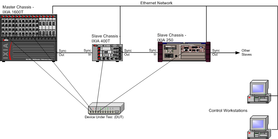
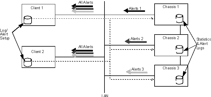
The following figure is a representation of an independent Ixia chassis chain and control network. Chassis are chained together through their sync cables. The first chassis in a chain has a Sync-out connection (but no Sync-in unless it is the AFD1 GPS receiver), and is called the master chassis. All other chassis in the chain are termed subordinates.
Figure 2-1. Ixia Chassis Chain and Control Workstation
Multiple, geographically-separated, independent chassis may be synchronized with a high degree of accuracy by using an Ixia chassis. Specific chassis include an integral GPS or CDMA receiver which is used for worldwide chassis synchronization. See Chassis Synchronization on page 2-5 for a complete discussion of chassis timing.
Ports from the chassis are connected to the Device Under Test (DUT) using cables appropriate for the media. Ports from any chassis may be connected to the similar ports on the DUT. It is even possible to connect multiple independent DUTs to different ports on different chassis.
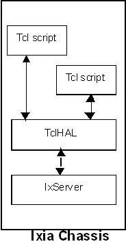
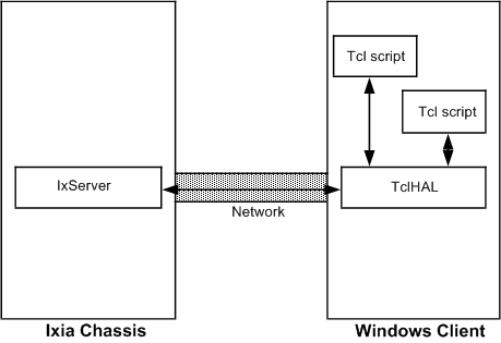
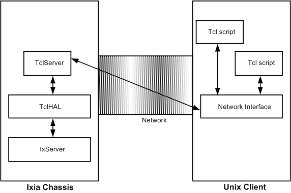
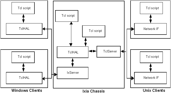
Each chassis is driven by an Intel Pentium-based computer running Windows XP Professional and Ixia-supplied software. Each chassis may be directly connected to a monitor, keyboard, and mouse to create a standalone system, but it is typical to connect all chassis through an Ethernet network and run the IxExplorer client software or Tcl client software on one or more external control PC workstations. IxExplorer client software runs on any Windows 2000/XP based system or Windows Server 2003 (console usage or simultaneous remote terminal access for multiple users). Tcl client software runs on Windows 2000/XP based systems and several Unix-based systems.
Chassis Chain Timing Specification
Based on the above numbers:
Chassis
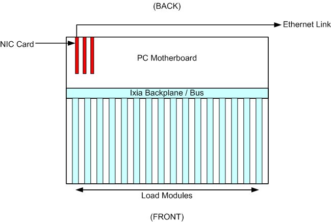
Each Ixia chassis can operate as a complete standalone system when connected to a local monitor, keyboard, and mouse. The interior of an Ixia 1600T chassis is shown in the following figure.
Figure 2-2. Ixia 1600T Interior View (Top View)
The PC embedded in the chassis system is an Intel-compatible computer system which includes the following components:
The Ixia Backplane is connected to the PC Motherboard, through an Ixia custom PCI interface card, and to the card slots where the Ixia load modules are installed.
Chassis Synchronization
Measurement of unidirectional latency and jitter in the transmission of data from a transmit port to a receive port requires that the relationship between time signatures at each of the ports is known. This can be accomplished by providing the following signals between chassis:
- Clock (frequency standard): This allows chassis to phase-lock their frequency standards so that a cycle counter on any chassis counts the same number of cycles during the same time interval. Each Ixia port maintains such a counter from a common chassis-wide frequency standard.
- Reset: A means must exist to either discover the fixed offset between their counters, or to simultaneously set the counters to a known value. You may think of this as the zero reset.
The use of both Reset and Phase Lock allow the establishment and maintenance of a fixed time reference between two or more chassis and the ports supported by the chassis.
In test setups where chassis and ports are physically close together, a sync cable is used to connect chassis in a `chassis chain' for synchronization operation.
In widely distributed applications, such as monitoring traffic characteristics over a WAN, clock reference and/or reset signals cannot be transmitted between chassis over a physical connection because of unknown delay characteristics. An alternative means is required to satisfy these requirements.
Ixia has facilities that allow for the synchronization of independent Ixia chassis located anywhere in the world by replacing the existing inter-chassis sync cables with a widely available frequency and time standard supplied from an external source. This source provides a reference time used to obtain accurate latency and other measurements in a live global network. When geographically dispersed chassis are connected in this way, the combination is called a virtual chassis chain.
Physical Chaining
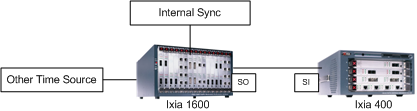
Independent Ixia 400T, 1600T, Optixia XL10, Optixia XM12, Optixia XM2, or Optixia X16 chassis may synchronize themselves with other chassis as shown in the following figure. The timing choices are explained in Table 2-2.
Figure 2-3. Physical Chaining
Virtual Chaining
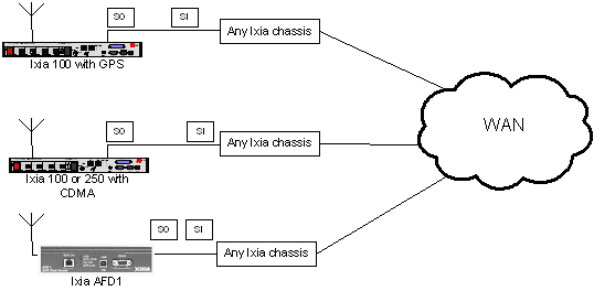
If two chassis are separated by any significant distance, a sync-out/sync-in cable cannot be used to connect them. In this case, either an Ixia Auxiliary Function Device (AFD1) or an Ixia 100 chassis with built-in Global Positioning Satellite (GPS), or an Ixia 100 or Ixia 250 with Code Division Multiple Access (CDMA) is used, one attached to each chassis through sync-out/sync-in cables, as shown in the following figure. The Ixia 100 maintains an accuracy of less than 150 nanoseconds when attached to a GPS antenna, or 100 microseconds when attached to a CDMA receiver, and provides chassis to chassis synchronization.
Figure 2-4. Virtual Chaining
To generate traffic for system latency testing, the Ixia 100 or Ixia 250 chassis can be used alone or in conjunction with another Ixia chassis, or the Ixia AFD1 (GPS receiver) can be used with any other Ixia chassis. The timing features available with these chassis are shown in Table 2-3 on page 2-7. A GPS antenna requires external mounting. Refer to Appendix C, GPS Antenna Installation Requirements for more information.
The Sync-Out from a GPS or CDMA chassis is used to master a chassis chain at a specific geographic location. Since the Ixia 100 or Ixia 250 chassis has all other functions provided by the other Ixia chassis, it may also use independent timing when not used to synchronize with other chassis at other locations.
For more information, including a formula for Calculating Latency Accuracy for AFD1 (GPS), see Chapter 19, Ixia GPS Auxiliary Function Device (AFD1).
Ixia Chassis Connections
A number of LEDs are available on the front panel of the Ixia 100 or Ixia 250, as described in Table 2-4 on page 2-8.
Similar information is available for the AFD1 GPS receiver in the Time Source tab of the Chassis Properties form (viewable through IxExplorer user interface).
Load Modules
Although each Ixia load module differs in particular capabilities, all modules share a common set of functions. Ixia load modules are generally categorized by network technology. The network technologies supported, along with names used to reference these technologies and more detailed information on load module differences, are available in the subsequent chapters of this manual.
The Load Module name prefix is used as the prefix to all load modules for that technology; for example, LM 100 in LM 100 TX. The IxExplorer name is used to label card and port types.
Some load modules are further labelled by the type of connector supported. Thus, a load module's name can be formed from a combination of its basic technology and the connector type. For example, LM 100 TX is the name of the 10/100 load module with RJ-45 connectors. An example for Packet Over SONET (POS) is the LMOC48c POS module, where no connector type is specified.
In addition, less expensive versions of several load modules are available. These are called Type-3 or Type-M modules, signified by an ending of `-3' or `-M' in the load module name and with a `-3'or `-M' suffix in the IxExplorer.
Newer boards also may have an `L' before the last number in their part number, signifying the same limited functionality (example: LSM10GL1-01).
Some load modules can be configured with less than standard amount of memory. Modules configured with such memory have a notation as to the memory upgrade following the module name. For example, LM622MR-512.
Port Hardware
The ports on the Ixia load modules provide high-speed, transmit, capture, and statistics operation. The discussion which follows is broken down into a number of areas:
- Types of Ports on page 2-9: The different types of networking technology supported by Ixia load modules
- Port Transmit Capabilities on page 2-47: Facilities for generating data traffic
- Streams and Flows: A set of packets, which may be grouped into bursts
- Bursts and the Inter-Burst Gap (IBG): A number of packets
- Packets and the Inter-Packet Gap (IPG): Individual frames/packets of data
- Frame Data on page 2-51: The construction of data within a frame/packet
- Port Data Capture Capabilities on page 2-66: Facilities for capturing data received on a port
- Port Statistics Capabilities on page 2-76: Facilities for obtaining statistics on each port
Types of Ports
The types of load module ports that Ixia offers are divided into these broad categories:
Only the currently available Ixia load modules are discussed in this chapter. Subsequent chapters in this manual discuss all supported load modules and their optional features.
Ethernet
Ethernet modules are provided with various feature combinations, as mentioned in the following list:
- Speed combinations: 10 Mbps, 100 Mbps, and 1000 Mbps
- Auto negotiation
- Pause control
- With and without on-board processors, also called Port CPUs (PCPUs). Load modules without processors only allow for very limited routing protocol emulation
- Power over Ethernet (Described in Power over Ethernet on page 2-10)
- External connections including the following:
Power over Ethernet
The Power over Ethernet (PoE) load modules (PLM1000T4-PD and LSM1000POE4-02) are special purpose, 4-channel electronic loads. They are intended to be used in conjunction with Ixia ethernet traffic generator/analyzer load modules to test devices that conform to IEEE std 802.3af.
A PoE load module provides the hardware interface required to test the Power Sourcing Equipment (PSE) of a 802.3af compliant device by simulating a Powered Device (PD).
Power Sourcing Equipment (PSE)
A PSE is any equipment that provides the power to a single link Ethernet Network section. The PSE's main functions are to search the link section for a powered device (PD), optionally classify the PD, supply power to the link section (only if a PD is detected), monitor the power on the link section, and remove power when it is no longer requested or required.
There are two power sourcing methods for PoE—Alternative A and Alternative B.
PSEs may be placed in two locations with respect to the link segment, either coincident with the DTE/Repeater, or midspan. A PSE that is coincident with the DTE/Repeater is an `Endpoint PSE.' A PSE that is located within a link segment that is distinctly separate from and between the Media Dependent Interfaces (MDIs) is a `Midspan PSE.'
Endpoint PSEs may support either Alternative A, B, or both. Endpoint PSEs can be compatible with 10BASE-T, 100BASE-X, and/or 1000BASE-T.
Midspan PSEs must use Alternative B. Midspan PSEs are limited to operation with 10BASE-T and 100BASE-TX systems. Operation of Midspan PSEs on 1000BASE-T systems is beyond the scope of PoE.
Powered Devices (PD)
A powered device either draws power or requests power by participating in the PD detection algorithm. A device that is capable of becoming a PD may or may not have the ability to draw power from an alternate power source and, if doing so, may or may not require power from the PSE.
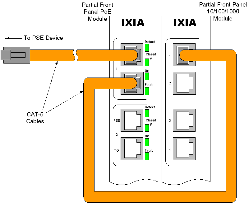
One PoE Load Module emulates up to four PDs. The PoE Load Module (PLM) has eight RJ-45 interfaces—four of them used as PD-emulated ports, with each having its own corresponding interface that connects to a port on any Ixia 10/100/1000 copper-based Ethernet load module (includes LM100TX, all copper-based TXS, and Optixia load modules).
The following figure demonstrates how the PoE modules use an Ethernet card to transmit and receive data streams.
Figure 2-5. Data Traffic over PoE Set Up
The emulated PD device can `piggy-back' a signal from a different load module along the cable connected to the PSE from which it draws power. In this manner, the emulated PD can mimic a device that generates traffic, such as an IP phone.
Discovery Process
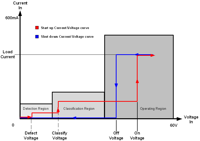
The main purpose for discovery is to prevent damage to existing Ethernet equipment. The Power Sourcing Equipment (PSE) examines the Ethernet cables by applying a small current-limited voltage to the cable and checking for the presence of a 25K ohm resistor in the remote Powered Device (PD). Only if the resistor is present, the full 48V is applied (and this is still current-limited to prevent damage to cables and equipment in fault conditions). The Powered Device must continue to draw a minimum current or the PSE removes the power and the discovery process begins again.
Figure 2-6. Discovery Process Voltage
There is also an optional extension to the discovery process where a PD may indicate to the PSE its maximum power requirements, called classification. Once there is power applied to the PD, normal transactions/data transfer occurs. During this period, the PD sends back a maintain power signature (MPS) to signal the PSE to continue to provide power.
PoE Acquisition Tests
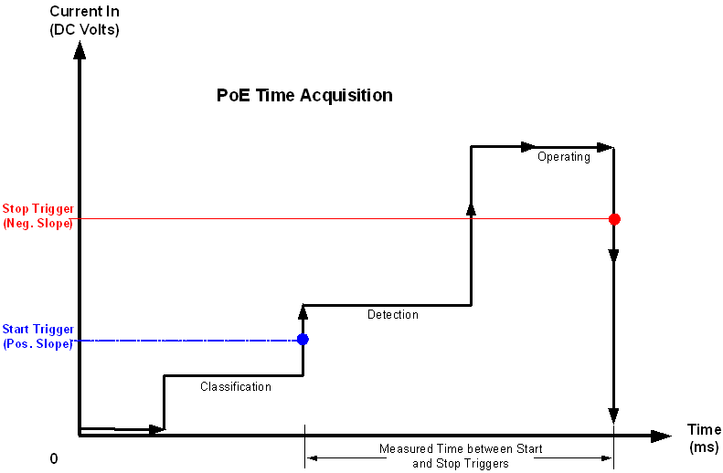
During the course of testing with the PoE module, it may be necessary to measure the amplitude of the incoming current. The PoE module has the ability to measure amplitude versus time in following two ways:
In both scenarios, a Start trigger is set, indicating when the test should commence based on an incoming current value (in either DC Volts or DC Amps).
In a Time test, a Stop trigger is also set (in either DC Volts or DC Amps) indicating when the test is over. Once the Stop trigger is reached, the amount of time between the Start and Stop trigger is measured (in microseconds) and the result is reported.
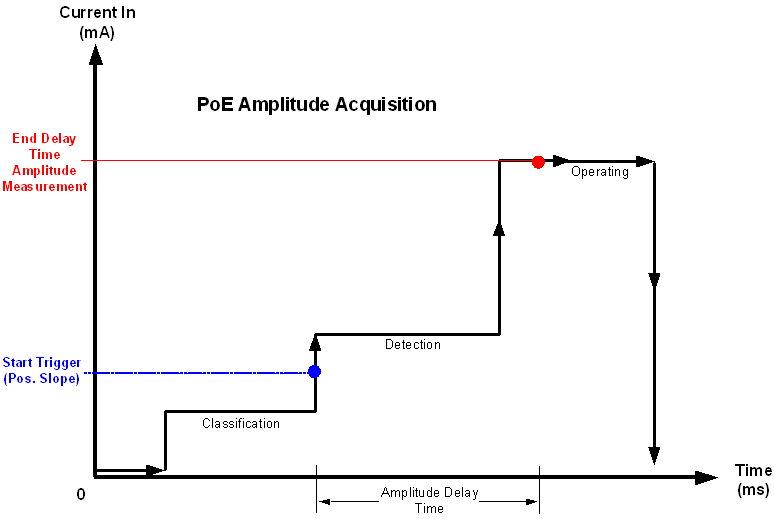
In an amplitude test, an Amplitude Delay time is set (in microseconds), which is the amount of time to wait after the Start trigger is reached before ending the test. The amplitude at the end of the Amplitude Delay time is measured and is reported.
Both Start and Stop triggers must also have a defined Slope type, either positive or negative. A positive slope is equivalent to rising current, while a negative slope is equivalent to decreasing current. A current condition must agree with both the amplitude setting and the Slope type to satisfy the trigger condition.
An example of a Time test is shown in the following figure, and an example of an Amplitude test is shown in Figure 2-8.
Figure 2-7. PoE Time Acquisition Example
Figure 2-8. PoE Amplitude Acquisition Example
10GE
The 10 Gigabit Ethernet (10GE) family of load modules implements five of the seven IEEE 8.2.3ae compliant interfaces that run at 10 Gbit/second. Several of the load modules may also be software switched to OC192 operation.
The 10 GE load modules are provided with various feature combinations, as mentioned in the following list:
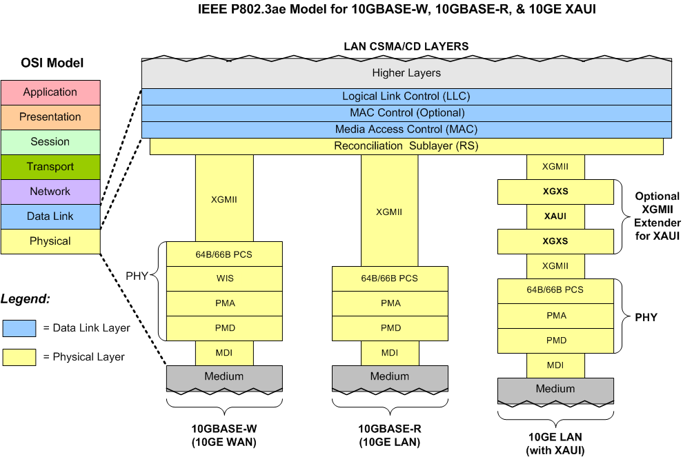
The relationship of the logical structures for the different 10 Gigabit types is shown in the diagram (adapted from the 802.3ae standard) in the following figure.
Figure 2-9. IEEE 802.3ae Draft—10 Gigabit Architecture
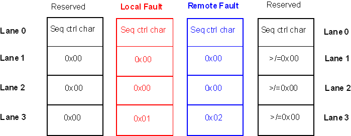
For 10GE XAUI and 10GE XENPAK modules, a Status message contains a 4-byte ordered set with a Sequence control character plus three data characters (in hex), distributed across the four lanes, as shown in the following figure. Four Sequence ordered sets are defined in IEEE 802.3ae, but only two of these—Local Fault and Remote Fault—are currently in use; the other two are reserved for future use.
Figure 2-10. 10GE XAUI/XENPAK Sequence Ordered Sets
XAUI Interfaces
The 10 Gigabit XAUI interface has been defined in the IEEE draft specification P802.3ae by the 10 Gigabit Ethernet Task Force (10GEA). XAUI stands for `X' (the Roman Numeral for 10, as in `10 Gigabit'), plus `AUI' or Attachment Unit Interface originally defined for Ethernet.
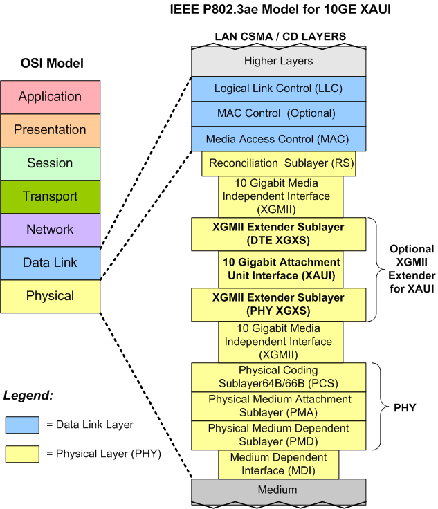
The original Ethernet standard was defined in IEEE 802.3, and included MAC layer, frame size, and other `standard' Ethernet characteristics. IEEE 802.3z defined the Gigabit standard. IEEE 802.3ae has been created to create a simplified version of SONET framing to carry native Ethernet-framed traffic over high-speed fiber networks. This new standard allows a smooth transition from 10 Gbps native Ethernet traffic to work with 9.6 Gbps for SONET at OC-192c rate over WAN and MAN links. The 10GE XAUI has a XAUI interface for connecting to another XAUI interface, such as on a DUT. A comparison of the IEEE P802.3ae model for XAUI and the OSI model is shown in the following figure.
Figure 2-11. IEEE P802.3ae Architecture for 10GE XAUI
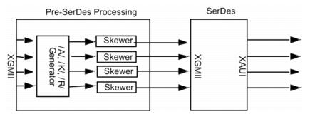
Lane Skew
The Lane Skew feature provides the ability to independently delay one or more of the four XAUI lanes. The resolution of the skew is 3.2 nanoseconds (ns), which consists of 10 Unit Intervals (UIs), each of which is 320 picoseconds (ps). Each UI is equivalent to the amount of time required to transmit one XAUI bit at 3.125 Gbps.
Lane Skew allows a XAUI lane to be skewed by as much as 310 UI (99.2ns) with respect to the other three lanes. To effectively use this feature, the four lanes should be set to different skew values. Setting all four lanes to zero is equivalent to setting all four lanes to +80 UI. In both cases, the lanes are synchronous and there is no lane skew. When lane skewing is enabled, /A/, /K/, and /R/ codes are inserted into the data stream BEFORE the lanes are skewed. The principle behind lane skewing is shown in the diagrams in Figure 2-12 and Figure 2-13.
Figure 2-12. XAUI Lane Skewing—Lane Skew Disabled
Figure 2-13. XAUI Lane Skewing—Lane Skew Enabled
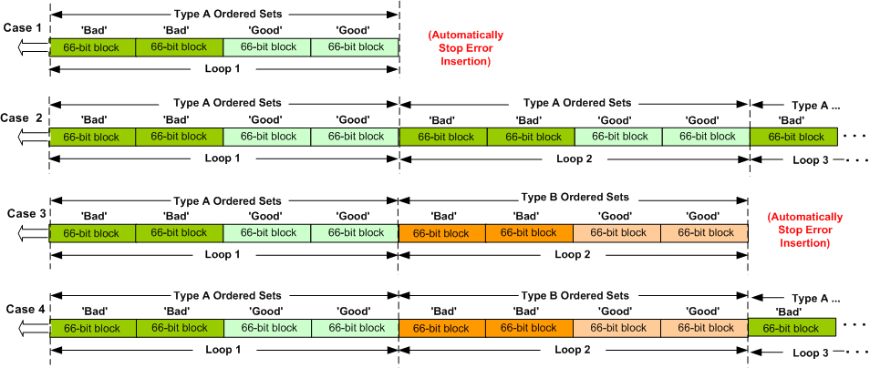
Link Fault Signaling
Link Fault Signaling is defined in Section 46 of the IEEE 802.3ae specification for 10 Gigabit Ethernet. When the feature is enabled, four statistics are added to the list in Statistic View for the port. One is for monitoring the Link Fault State; two for providing a count of the Local Faults and Remote Faults; and the last one is for indicating the state of error insertion, whether or not it is ongoing.
Link Fault Signaling originates with the PHY sending an indication of a local fault condition in the link being used as a path for MAC data. In the typical scenario, the Reconciliation Sublayer (RS) which had been receiving the data receives this Local Fault status, and then send a Remote Fault status to the RS which was sending the data. Upon receipt of this Remote Fault status message, the sending RS terminates transmission of MAC Data, sending only `Idle' control characters until the link fault is resolved.
For the 10GE LAN and LAN-M serial modules, the Physical Coding Sublayer (PCS) of the PHY handles the transition from 64 bits to 66 bit `Blocks.' The 64 bits of data are scrambled, and then a 2-bit synchronization (sync) header is attached before transmission. This process is reversed by the PHY at the receiving end.
Link Fault Signaling for the 10GE XAUI/XENPAK is handled differently across the four-lane XAUI optional XGMII extender layer, which uses 8B/10B encoding.
Figure 2-14. Examples of Link Fault Signaling Error Insertion
The examples in this figure are described in the following table:
Link Alarm Status Interrupt (LASI)
The link alarm status is an active low output from the XENPAK module that is used to indicate a possible link problem as seen by the transceiver. Control registers are provided so that LASI may be programmed to assert only for specific fault conditions.
Efficient use of XENPAK and its specific registers requires an end-user system to recognize a connected transceiver as being of the XENPAK type. An Organizationally Unique Identifier (OUI) is used as the means of identifying a port as XENPAK, and also to communicate the device in which the XENPAK specific registers are located.
Ixia's XENPAK module allows for setting whether or not LASI monitoring is enabled, what register configurations to use, and the OUI. The XENPAK module can use the following registers:
- Rx Alarm Control (Register 0x9003): It can be programmed to assert only when specific receive path fault condition(s) are present.
- Tx Alarm Control (Register 0x9001): It can be programmed to assert only when specific transmit path fault condition(s) are present.
- LASI Control (Register 0x9002): A LASI control register that allows global masking of the Rx Alarm and Tx Alarm.
You can control the registers by setting a series of sixteen bits for each register. The register bits and their usage are described in the following tables.
For more detailed information on LASI, see the online document XENPAK MSA Rev. 3.
40GE and 100GE
For theoretical information, refer to 40 Gigabit Ethernet and 100 Gigabit Ethernet Technology Overview White Paper, published by Ethernet Allliance, November, 2008. This white paper may be obtained through the Internet.
http://www.ethernetalliance.org/images/40G_100G_Tech_overview.pdf
SONET/POS
SONET/POS modules are provided with various feature combinations:
- Different speeds: OC3, OC12, OC48, OC192, Fibre Channel, 2x Fibre Channel, and Gigabit Ethernet.
- Interfaces: SC singlemode and multimode (OC3, OC12, OC192), SC singlemode (OC48), no optical transceiver, SFP LC singlemode (Unframed BERT) and custom interface.
- Reach: long, intermediate and long.
- Wavelengths: 850nm, 1310nm and 1550nm.
- Local processor support. All SONET/POS load modules include a local processor, but the power of the processor and amount of memory varies.
- Variable clocking—OC48 only, see Variable Rate Clocking on page 2-22.
- Concatenated or channelized SONET operation, see SONET Operation on page 2-22.
- Error insertion, see Error Insertion on page 2-24.
- BERT: Bit Error Rate Testing both framed and unframed, see BERT on page 2-45.
- DCC: Data Communication Channel, see DCC—Data Communications Channel on page 2-25.
- RPR: Resilient Packet Ring, see RPR—Resilient Packet Ring on page 2-26.
- GFP: Generic Framing Procedure, see GFP—Generic Framing Procedure on page 2-29.
- PPP: Point to Point protocol, see PPP Protocol Negotiation on page 2-33.
- HDLC: High-Level Data Link Control, see HDLC on page 2-39.
- Frame Relay: see Frame Relay on page 2-39.
Variable Rate Clocking
The OC48 VAR allows a variation of +/- 100 parts per million (ppm) from the clock source's nominal frequency, through a DC voltage input into the BNC jack marked `DC IN' on the front panel. The frequency may be monitored through the BNC marked `Freq Monitor.'
SONET Operation
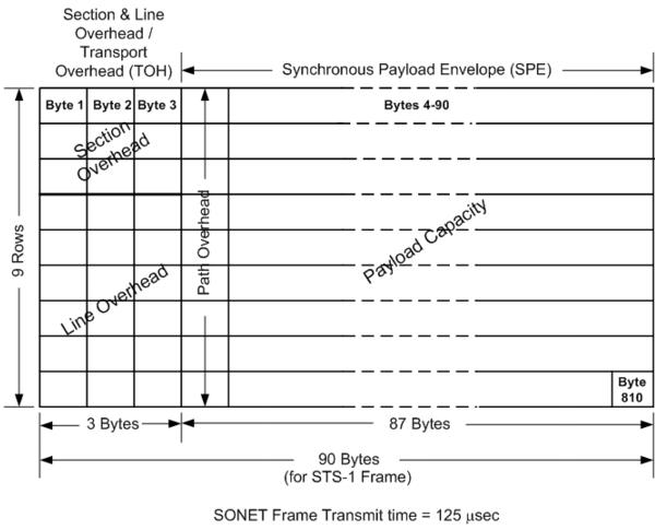
A Synchronous Optical NETwork/Synchronous Digital Hierarchy (SONET/SDH) frame is based on the Synchronous Transport Signal-1 (STS-1) frame, whose structure is shown in Figure 2-15 on page 2-23. Transmission of SONET Frames of this size correspond to the Optical Carrier level 1 (OC-1).
An OC-3c, consists of three OC-1/STS-1 frames multiplexed together at the octet level. OC-12c, OC-48c, and OC-192c, are formed from higher multiples of the basic OC-1 format. The suffix `c' indicates that the basic frames are concatenated to form the larger frame.
Ixia supports both concatenated (with the `c') and channelized (without the `c') interfaces. Concatenated interfaces send and receive data in a single streams of data. Channelized interfaces send and receive data in multiple independent streams.
Figure 2-15. Generated Frame Contents—SONET STS-1 Frame
The contents of the SONET STS-1 frame are described in Table 2-9 on page 2-23.
The SONET STS-1 frame is transmitted at a rate of 51.84 Mbps, with 49.5 Mbps reserved for the frame payload. A SONET frame is transmitted in 125 microseconds, with the order of transmission of the starting with Row 1, Byte 1 at the upper left of the frame, and proceeding by row from top to bottom, and from left to right.
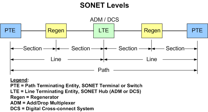
The section, line, and path overhead elements are related to the manner in which SONET frames are transmitted, as shown in Figure 2-16 on page 2-24.
Figure 2-16. Example Diagram of SONET Levels and Network Elements
Error Insertion
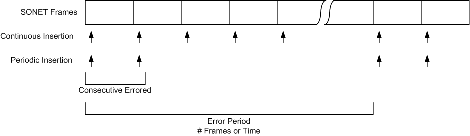
A variety of deliberate errors may be inserted in SONET frames in the section, line or path areas of a frame. The errors which may be inserted vary by particular load module. Errors may be inserted continuously or periodically as shown in Figure 2-17 on page 2-25.
Figure 2-17. SONET Error Insertion
An error may be inserted in one of two manners:
Each error may be individually inserted continuously or periodically. Errors may be inserted on a one time basis over a number of frames as well.
DCC—Data Communications Channel
The data communication channel is a feature of SONET networks which uses the DCC bytes in the transport overhead of each frame. This is used for control, monitoring and provisioning of SONET connections. Ixia ports treat the DCC as a data stream which `piggy-backs' on the normal SONET stream. The DCC and normal (referred to as the SPE - Synchronous Payload Envelope) streams can be transmitted independently or at the same time.
A number of different techniques are available for transmitting DCC and SPE data, utilizing Ixia streams and flows (see Streams and Flows on page 2-47) and advanced stream scheduler (see Advanced Streams on page 2-48).
SRP—Spatial Reuse Protocol
The Spatial Reuse Protocol (SRP) was developed by Cisco for use with ring-based media. It derives its name from the spatial reuse properties of the packet handling procedure. This optical transport technology combines the bandwidth-efficient and service-rich capabilities of IP routing with the bandwidth-rich, self-healing capabilities of fiber rings to deliver fundamental cost and functionality advantages over existing solutions. In SRP mode, the usual POS header (PPP, and so forth) is replaced by the SRP header.
SRP networks use two counter-rotating rings. One Ixia port may be used to participate in one of the rings; two may be used to simultaneously participate in both rings. Ixia supports SRP on both OC48 and OC192 interfaces.
In SRP-mode, SRP packets can be captured and analyzed. The IxExplorer capture view displays packet analysis which understands SRP packets. The Ixia hardware also collects specific SRP related statistics and performs filtering based on SRP header contents.
Any of the following SRP packet types may be generated in a data stream, along with normal IPv4 traffic:
RPR—Resilient Packet Ring
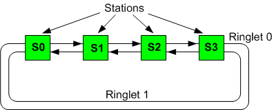
Ixia's optional Resilient Packet Ring (RPR) implementation is available on the OC-48c and OC-192c POS load modules. RPR is a proposed industry standard for MAC Control on Metropolitan Area Networks (MANs), defined by IEEE P802.17. This feature provides a cost-effective method to optimize the transport of bursty traffic, such as IP, over existing ring topologies.
A diagram showing a simplified model of an RPR network is shown in Figure 2-18 on page 2-26. It is made up of two, counter-rotating `ringlets,' with nodes called `stations' supporting MAC Clients that exchange data and control information with remote peers on the ring. Up to 255 nodes can be supported on the ring structure.
Figure 2-18. RPR Ring Network Diagram
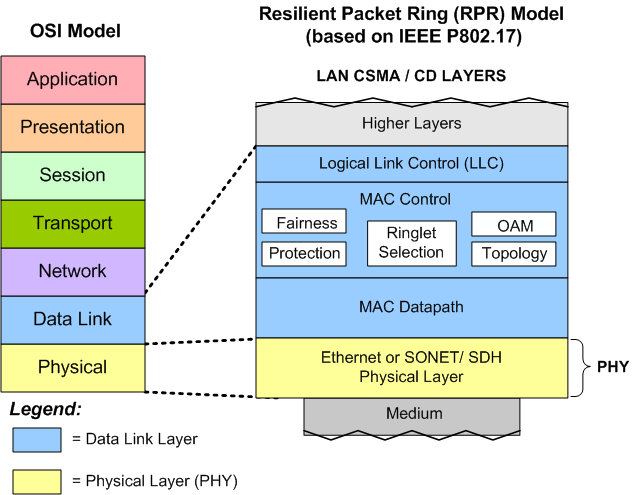
The RPR topology discovery is handled by a MAC sublayer, and a protection function maintains network connectivity in the event of a station or span failure. The structure of the RPR layers, compared to the OSI model, is illustrated in a diagram based on IEEE 802.17, shown in Figure 2-19 on page 2-27.
Figure 2-19. RPR Layers
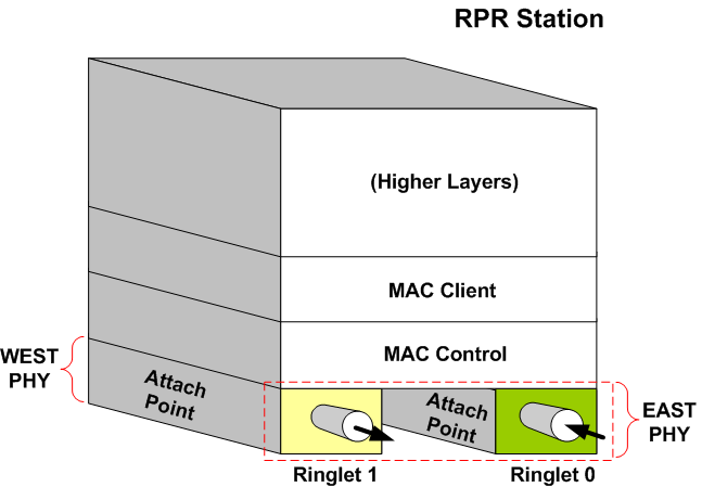
A diagram of the layers associated with an RPR Station is shown in Figure 2-20 on page 2-27.
Figure 2-20. RPR Layer Diagram
The Ixia implementation allows for the configuration and transmission of the following types of RPR frames:
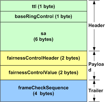
- RPR Fairness Frames: The RPR Fairness Algorithm (FA) is used to manage congestion on the ringlets in an RPR network. Fairness frames are sent periodically to advertise bandwidth usage parameters to other nodes in the network to maintain weighted fair share distributions of bandwidth. The messages are sent in the direction opposite to the data flow, and therefore, on the other ringlet. A diagram of the RPR Fairness Frame, per IEEE 802.17/D2.1, is shown in Figure 2-21 on page 2-28.
Figure 2-21. RPR Fairness Frame Format
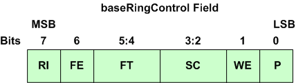
A diagram of the baseRingControl byte, part of the Ring Control header for all types of RPR frames, is shown in Figure 2-22 on page 2-28.
Figure 2-22. RPR baseRingControl Byte
- RPR Topology Discovery. Two types of messages are used:
- RPR Protection Switching Message: used to support automatic, rapid switching of traffic in the presence of a ring failure.
- RPR Operations, Administration and Management (OAM). Three messages are supported:
GFP—Generic Framing Procedure
GFP provides a generic mechanism to adapt traffic from higher-layer client signals over a transport network. Currently, two modes of client signal adaptation are defined for GFP.
In the Frame-Mapped adaptation mode, the Client/GFP adaptation function operates at the data link (or higher) layer of the client signal. Client PDU visibility is required, which is obtained when the client PDUs are received from either the data layer network or a bridge, switch, or router function in a transport network element.
For the Transparent adaptation mode, the Client/GFP adaptation function operates on the coded character stream, rather than on the incoming client PDUs. Processing of the incoming code word space for the client signal is required.
Two kinds of GFP frames are defined: GFP client frames and GFP control frames. GFP also supports a flexible (payload) header extension mechanism to facilitate the adaptation of GFP for use with diverse transport mechanisms.
GFP uses a modified version of the Header Error Check (HEC) algorithm to provide GFP frame delineation. The frame delineation algorithm used in GFP differs from HEC in two basic ways:
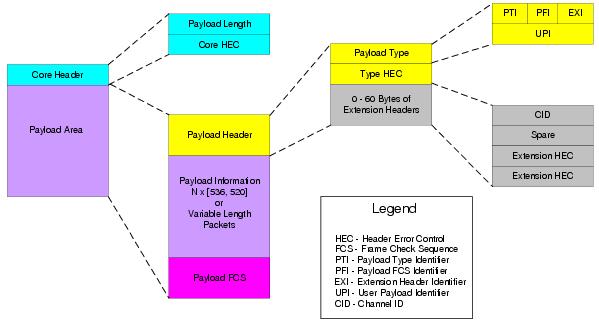
A diagram of the format for a GFP frame is shown in Figure 2-23 on page 2-30.
Figure 2-23.
GFP Frame Elements
The sections of the GFP frame are described in the following list:
- Payload Length Indicator (PLI): The two-octet PLI field contains a binary number representing the number of octets in the GFP Payload Area. The absolute minimum value of the PLI field in a GFP client frame is 4 octets. PLI values 0-3 are reserved for GFP control frame usage.
- Core Header Error Control (cHEC): The two-octet Core Header Error Control field contains a CRC-16 error control code that protects the integrity of the contents of the Core Header by enabling both single-bit error correction and multi-bit error detection.
- Type Header Error Control (tHEC): The two-octet Type Header Error Control field contains a CRC-16 error control code that protects the integrity of the contents of the Type field by enabling both single-bit error correction and multi-bit error detection.
- Extension Header Error Control (eHEC): The two-octet Extension Header Error Control field contains a CRC-16 error control code that protects the integrity of the contents of the extension headers by enabling both single-bit error correction (optional) and multi-bit error detection.
- Connection Identification (CID): The CID is an 8-bit binary number used to indicate one of 256 communications channels at a GFP termination point.
- Payload: The GFP Payload Area, which consists of all octets in the GFP frame after the GFP Core Header, is used to convey higher layer specific protocol information. This variable length area may include from 4 to 65,535 octets. The GFP Payload Area consists of two common components:
- Frame Check Sequence (FCS): The GFP Payload FCS is an optional, four-octet long, frame check sequence. It contains a CRC-32 sequence that protects the contents of the GFP Payload Information field. A value of 1 in the PFI bit within the Type field identifies the presence of the payload FCS field.
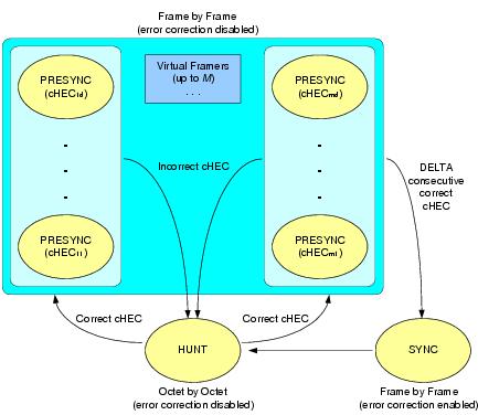
GFP frame delineation is performed based on the correlation between the first two octets of the GFP frame and the embedded two-octet cHEC field. Figure 2-24 on page 2-31 shows the state diagram for the GFP frame delineation method.
Figure 2-24.
GFP State Transitions
The state diagram works as follows:
- In the HUNT state, the GFP process performs frame delineation by searching octets for a correctly formatted Core Header over the last received sequence of four octets. Once a correct cHEC match is detected in the candidate Payload Length Indicator (PLI) and cHEC fields, a candidate GFP frame is identified and the receive process enters the PRESYNC state.
- In the PRESYNC state, the GFP process performs frame delineation by checking frames for a correct cHEC match in the presumed Core Header of the next candidate GFP frame. The PLI field in the Core Header of the preceding GFP frame is used to find the beginning of the next candidate GFP frame. The process repeats until a set number of consecutive correct cHECs are confirmed, at which point the process enters the SYNC state. If an incorrect cHEC is detected, the process returns to the HUNT state.
- In the SYNC state, the GFP process performs frame delineation by checking for a correct cHEC match on the next candidate GFP frame. The PLI field in the Core Header of the preceding GFP frame is used to find the beginning of the next candidate GFP frame. Frame delineation is lost whenever multiple bit errors are detected in the Core Header by the cHEC. In this case, a GFP Loss of Frame Delineation event is declared, the framing process returns to the HUNT state, and a client Server Signal Failure (SSF) is indicated to the client adaptation process.
- Idle GFP frames participate in the delineation process and are then discarded.
Robustness against false delineation in the resynchronization process depends on the value of DELTA. A value of DELTA = 1 is suggested. Frame delineation acquisition speed can be improved by the implementation of multiple `virtual framers,' whereby the GFP process remains in the HUNT state and a separate PRESYNC substate is spawned for each candidate GFP frame detected in the incoming octet stream.
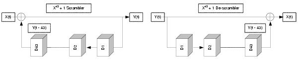
Scrambling of the GFP Payload Area is required to provide security against payload information replicating scrambling word (or its inverse) from a frame synchronous scrambler (such as those used in the SDH RS layer or in an OTN OPUk channel). Figure 2-25 on page 2-32 illustrates the scrambler and descrambler processes.
Figure 2-25. GFP Scrambling
All octets in the GFP Payload Area are scrambled using a x43 + 1 self-synchronous scrambler. Scrambling is done in network bit order.
At the source adaptation process, scrambling is enabled starting at the first transmitted octet after the cHEC field, and is disabled after the last transmitted octet of the GFP frame. When the scrambler or descrambler is disabled, its state is retained. Hence, the scrambler or descrambler state at the beginning of a GFP frame Payload Area is, thus, the last 43 Payload Area bits of the GFP frame transmitted in that channel immediately before the current GFP frame.
The activation of the sink adaptation process descrambler also depends on the present state of the cHEC check algorithm:
CDL— Converged Data Link
10GE LAN, 10GE XAUI, 10GE XENPAK, 10GE WAN, and 10GE WAN UNIPHY modules all support the Cisco CDL preamble format.
The Converged Data Link (CDL) specification was developed to provide a standard method of implementing operation, administration, maintenance, and provisioning (OAM&P) in Ethernet packet-based optical networks without using a SONET/SDH layer.
PPP Protocol Negotiation
The Point-to-Point Protocol (PPP) is widely used to establish, configure and monitor peer-to-peer communication links. A PPP session is established in a number of steps, with each step completing before the next one starts. The steps, or layers, are:
- Physical: a physical layer link is established.
- Link Control Protocol (LCP): establishes the basic communications parameters for the line, including the Maximum Receive Unit (MRU), type of authentication to be used and type of compression to be used.
- Link quality determination and authentication. These are optional processes. Quality determination is the responsibility of PPP Link Quality Monitoring (LQM) Protocol. Once initiated, this process may continue throughout the life of the link. Authentication is performed at this stage only. There are multiple protocols which may be employed in this process; the most common of these are PAP and CHAP.
- Network Control Protocol (NCP): establishes which network protocols (such as IP, OSI, MPLS) are to be carried over the link and the parameters associated with the protocols. The protocols which support this NCP negotiation are called IPCP, OSINLCP, and MPLSCP, respectively.
- Network traffic and sustaining PPP control. The link has been established and traffic corresponding to previously negotiated network protocols may now flow. Also, PPP control traffic may continue to flow, as may be required by LQM, PPP keepalive operations, and so forth.
All implementations of PPP must support the Link Control Protocol (LCP), which negotiates the fundamental characteristics of the data link and constitutes the first exchange of information over an opening link. Physical link characteristics (media type, transfer rate, and so forth) are not controlled by PPP.
The Ixia PPP implementation supports LCP, IPCP, MPLSCP, and OSINLCP. When PPP is enabled on a given port, LCP and at least one of the NCPs must complete successfully over that port before it is administratively `up' and therefore be ready for general traffic to flow.
Each Ixia POS port implements a subset of the LCP, LQM, and NCP protocols. Each of the protocols is of the same basic format. For any connection, separate negotiations are performed for each direction. Each party sends a Configure-Request message to the other, with options and parameters proposing some form of configuration. The receiving party may respond with one of three messages:
- Configure-Reject: The receiving party does not recognize or prohibits one or more of the suggested options. It returns the problematic options to the sender.
- Configure-NAK: The receiving party understands all of the options, but finds one or more of the associated parameters unacceptable. It returns the problematic options, with alternative parameters, to the sender.
- Configure-ACK: The receiving party finds the options and parameters acceptable.
For the Configure-Reject and Configure-NAK requests, the sending party is expected to reply with an alternative Configure-Request.
The Ixia port may be configured to immediately start negotiating after the physical link comes up, or passively wait for the peer to start the negotiation. Ixia ports both sends and responds to PPP keepalive messages called echo requests.
LCP—Link Control Protocol Options
The following sections outline the parameters associated with the Link Control Protocol. LCP includes a number of possible command types, which are assigned option numbers in the pertinent RFCs. Note that PPP parameters are typically independently negotiated for each direction on the link.
Numerous RFCs are associated with LCP, but the most important RFCs are RFC 1661 and RFC 1662. The HDLC/PPP header sequence for LCP is FF 03 C0 21.
During the LCP phase of negotiation, the Ixia port makes available the following options:
- Maximum Receive Unit: This LCP parameter (actually the set of Maximum Receive Unit (MRU) and Maximum Transmit Unit (MTU)) determines the maximum allowed size of any frame sent across the link subsequent to LCP completion. To be fully standards-compliant, an implementation must not send a frame of length greater than its MTU + 4 bytes + CRC length. For instance, if the negotiated MTU for a port is 2000 and 32 bit CRC is in use, no frame larger than 2008 bytes should ever be sent out that port. Packets that are larger are expected to be fragmented before transmitting or to be dropped. The Ixia port's MTU is the peer's MRU following LCP negotiation. Strictly speaking, the receiving side can assume that frames received is not greater than the MRU. In practice, however, an implementation should be capable of accepting larger frames. If a peer rejects this option altogether, the negotiated setting defaults to 1,500. Regardless of the negotiated MRU, all implementations must be capable of accepting frames with an information field of at least 1,500 bytes.
For the transmit direction portion of the negotiation, the peer sends the Ixia port its configuration request. The Ixia port accepts and acknowledges the peer's requested MRU as long as it is less than or equal to the specified user's desired transmit value (but greater than 26). For the receive direction portion of the negotiation, the Ixia port sends a configuration request based on the user's desired value. Generally, the Ixia port accepts what the peer desires (if it acknowledges the request, then the user value is used, or if the peer sends a Configure-Nak with another value the Ixia port uses that value as long as it is valid). This approach is used to maximize the probability of successful negotiation.
- Asynchronous Control Character Map: ACCM is only really pertinent to asynchronous links. On asynchronous lines, certain characters sent over the wire can have special meaning to one or more receiving entities. For instance, common implementations of the widely used XON/XOFF flow control protocol assign the ASCII DC3 character (0x13) to XOFF. On such a link, an embedded data byte that happens to have the value 0x13 would be misinterpreted by a receiver as an XOFF command, and cause suspension of reception. To avoid this problem, the 0x13 character embedded in the data could be sent through an `escape sequence' which consists of preceding the data character with a dedicated tag character and modifying the data character itself.
The Asynchronous Control Character Map (ACCM) LCP parameter allows independent designation of each character in the range 0x00 thru 0x1F as a control character. A control character is sent/received with a preceding `control-escape' character (0x7D). When the 0x7D is seen in the received data stream, the 0x7D is dropped and the next character is exclusive-or'd with 0x20 to get the original transmitted character. ACCM negotiation consists of exchanging masks between peers to reach an agreement as to which characters are treated as special control characters on transmission and reception. For example, sending a mask of 0xFFFFFFFF means all characters in the range 0x00 thru 0x1F are sent with escape sequences; a mask of 0 means no special handling, so all characters are arbitrary data.
Packet over SONET is an octet-synchronous medium. If the link is direct between POS peers, neither side should be generating control-escapes. (Exceptions to this are bytes 0x7D and 0x7E: the former is the special control escape character itself; the latter is the start/end frame marker. Escaping of these two characters is generally handled directly by physical layer hardware). On links in which there is some kind of intermediate asynchronous media, it is required that whatever device performs the asynchronous to synchronous conversion must also take care of any special character handling, isolating this from any POS port. See RFC 1662, sections 4.1 and 6.
If ACCM negotiation is enabled, the Ixia port advertises an ACCM mask of 0 to its peer in its LCP configuration request. The Ixia port accept whatever the peer puts forth, but does not act on the results. Regardless of the final negotiated settings for receive and transmit ACCM, the Ixia port does not send escape control sequences nor does it expect to receive them. This is the nature of a synchronous PPP medium, such as POS.
- Magic Number: A magic number is a 32-bit value, ideally numerically random, which is placed in certain PPP control packets. Magic numbers aid in detection of looped links. If a received PPP packet that includes a magic number matches a previously transmitted packet, including magic number, the link is probably looped.
IxExplorer and the Tcl APIs allow global enable/disable of magic number negotiation. If the `Use Magic Number' feature is enabled, the Ixia port does not request magic number of its peer and rejects the option if the peer requests it. If the check box is selected, the port attempts to negotiate magic number. The result of the bi-directional negotiation process is displayed in the fields for transmit and receive: an indication of whether magic number is enabled is written in the field for the corresponding direction.
NCP—Network Control Protocols
- IPCP: Internet Protocol Control Protocol Options for IPV4. IPCP includes three command types, which are assigned option numbers in the pertinent RFCs. Note that PPP parameters are typically independently negotiated for each direction on the link.
The sender of this Configure-Request may either include its own IP address, to provide this information to its remote peer, or may send all 0.0.0.0 as an IP address, which requests that the remote peer assign an IP address for the local node. The receiver may refuse the requested IP address and attempt to specify one for the peer to use by using a Configure-NAK response to the request with a specification of a different address.
The Ixia implementation provides minimal configuration of this parameter. You must specify the local IP address of the unit and the peer must provide its own IP address. The Ixia port accepts any IP address the peer wishes to use as long as it is a valid address (for example, not all 0's). The Ixia port expects the peer to accept its address. If, however, the peer specifies a different address for use, the port acknowledges that address but not actually notify you that this has happened. The Ixia port accepts a situation in which local and peer addresses are the same following negotiation.
- IPv6CP: Internet Protocol Control Protocol Options for IPv6. IPv6CP includes three command types, which are assigned option numbers in the pertinent RFCs. Note that PPP parameters are typically independently negotiated for each direction on the link.
A PPP peer may determine its IPv6 interface address by one or three methods:
- Generate its own address.
- Suggest its own address to its peer, but allow the peer to override that value.
- Require that the peer designate an address.
In any of these cases, the Configure-Request must contain a tentative interface-identifier to send to the peer that is both unique to the link and if possible consistently reproducible.
The Ixia PPP implementation of IPv6CP is such that the negotiation mode of the local endpoint may be configured in one of three modes:
- Local may: the local peer may suggest an Interface Identifier (IID), but most allow a Configure-NAK with an alternate address to override its setting.
- Local must: the local peer must set the IID, which the peer must accept.
- Peer must: the peer must supply the IID. This is accomplished by sending an all zero tentative IID.
The peer endpoint may be configured in one of three modes:
- Peer may: the remote peer may suggest an IID, but most allow a Configure-NAK with an alternate address to override its setting.
- Peer must: the remote peer must set the IID, which the local peer accepts.
- Local must: the local peer must supply the IID.
One IID can be sent in each Configuration-Request. A zero value may be sent, in which case, the peer may send an IID in its response. Either node on the link can provide the valid, non-zero IID values for itself and its peer.
The tentative, or assigned IID in the Peer - Local Must case, may be assigned from one of four sources:
- Last Negotiated: the last negotiated interface-identifier.
- MAC Based: an address derived from the port's MAC address.
- IPv6: an IPv6 format address.
- Random: a randomly generated value.
See IPv6 Interface Identifiers as follows for more information.
- OSI Network Layer Control Protocol (OSINLCP): A single option is provided for this NCP protocol. If a non-zero value for alignment has been negotiated, subsequent ISO traffic (for example, IS-IS) arrives with or be sent with 1 to 3 zero pads inserted after the protocol header as per RFC 1377.
- MPLS Network Control Protocol (MPLSCP): No options are currently available for this protocol setup.
IPv6 Interface Identifiers (IIDs)
IIDs comprise part of an IPv6 address, as shown in Figure 2-26 on page 2-38 for a link-local IPv6 address.
Figure 2-26. IPv6 Address Format—Link-Local Address
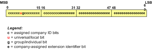
The IPv6 Interface Identifier is derived from the 48-bit IEEE 802 MAC address or the 64-bit IEEE EUI-64 identifier. The EUI-64 is the extended unique identifier formed from the 24-bit company ID assigned by the IEEE Registration Authority, plus a 40-bit company-assigned extension identifier, as shown in Figure 2-27 on page 2-38
Figure 2-27. IEEE EUI-64 Format
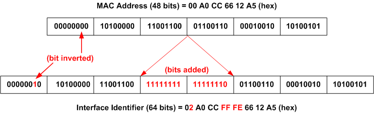
To create the Modified EUI-64 Interface Identifier, the value of the universal/local bit is inverted from `0' (which indicates global scope in the company ID) to `1' (which indicates global scope in the IPv6 Identifier). For Ethernet, the 48-bit MAC address may be encapsulated to form the IPv6 Identifier. In this case, two bytes `FF FE' are inserted between the company ID and the vendor-supplied ID, and the universal/local bit is set to `1' to indicate global scope. An example of an Interface Identifier based on a MAC address is shown in Figure 2-28 on page 2-39.
Figure 2-28. Example—Encapsulated MAC in IPv6 Interface Identifier
Retry Parameters
During the process of negotiation, the port uses three Retry parameters. RFC 1661 specifies the interpretation for all of the parameters.
HDLC
Both standard and Cisco proprietary forms of HDLC (High-level Data Link Control) are supported.
Frame Relay
Packets may be wrapped in frame relay headers. The DLCI (Data Link Connection Identifier) may be set to a fixed value or varied algorithmically.
DSCP—Differentiated Services Code Point
Differentiated Services (DiffServ) is a model in which traffic is treated by intermediate systems with relative priorities based on the type of services (ToS) field. Defined in RFC 2474 and RFC 2475, the DiffServ standard supersedes the original specification for defining packet priority described in RFC 791. DiffServ increases the number of definable priority levels by reallocating bits of an IP packet for priority marking.
The DiffServ architecture defines the DiffServ (DS) field, which supersedes the ToS field in IPv4 to make Per-Hop Behavior (PHB) decisions about packet classification and traffic conditioning functions, such as metering, marking, shaping, and policing.
Based on DSCP or IP precedence, traffic can be put into a particular service class. Packets within a service class are treated the same way.
The six most significant bits of the DiffServ field are called the Differential Services Code Point (DSCP).
The DiffServ fields in the packet are organized as shown in Figure 2-29 on page 2-40. These fields replace the TOS fields in the IP packet header.
Figure 2-29.
DiffServ Fields
The DiffServ standard utilizes the same precedence bits (the most significant bits are DS5, DS4, and DS3) as TOS for priority setting, but further clarifies the definitions, offering finer granularity through the use of the next three bits in the DSCP. DiffServ reorganizes and renames the precedence levels (still defined by the three most significant bits of the DSCP) into these categories (the levels are explained in greater detail in this document). Figure 2-10 on page 2-40 shows the eight categories.
With this system, a device prioritizes traffic by class first. Then it differentiates and prioritizes same-class traffic, taking the drop probability into account.
The DiffServ standard does not specify a precise definition of `low,' `medium,' and `high' drop probability. Not all devices recognize the DiffServ (DS2 and DS1) settings; and even when these settings are recognized, they do not necessarily trigger the same PHB forwarding action at each network node. Each node implements its own response based on how it is configured.
Assured Forwarding (AF) PHB group is a means for a provider DS domain to offer different levels of forwarding assurances for IP packets received from a customer DS domain. Four AF classes are defined, where each AF class is in each DS node allocated a certain amount of forwarding resources (buffer space and bandwidth).
Classes 1 to 4 are referred to as AF classes. The following table illustrates the DSCP coding for specifying the AF class with the probability. Bits DS5, DS4, and DS3 define the class, while bits DS2 and DS1 specify the drop probability. Bit DS0 is always zero.
ATM
The ATM load module enables high performance testing of routers and broadband aggregation devices such as DSLAMs and PPPoE termination systems.
The ATM module is provided with various feature combinations:
ATM is a point-to-point, connection-oriented protocol that carries traffic over `virtual connections/circuits' (VCs), in contrast to Ethernet connectionless LAN traffic. ATM traffic is segmented into 53-byte cells (with a 48-byte payload), and allows traffic from different Virtual Circuits to be interleaved (multiplexed). Ixia's ATM module allows up to 4096 transmit streams per port, shared across up to 15 interleaved VCs.
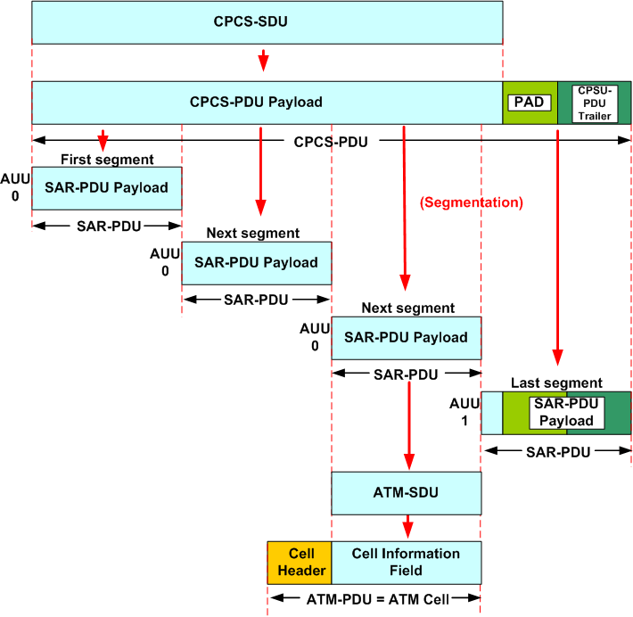
To allow the use of a larger, more convenient payload size, such as that for Ethernet frames, ATM Adaptation Layer 5 (AAL5) was developed. It is defined in ITU-T Recommendation I.363.5, and applies to the Broadband Integrated Services Digital Network (B-ISDN). It maps the ATM layer to higher layers. The Common Part Convergence Sublayer-Service Data Unit (CPSU-SDU) described in this document can be considered an IP or Ethernet packet. The entire CPSU-PDU (CPCS-SDU plus PAD and trailer) is segmented into sections which are sent as the payload of ATM cells, as shown in Figure 2-30 on page 2-42, based on ITU-T I.363.5.
Figure 2-30. Segmentation into ATM Cells
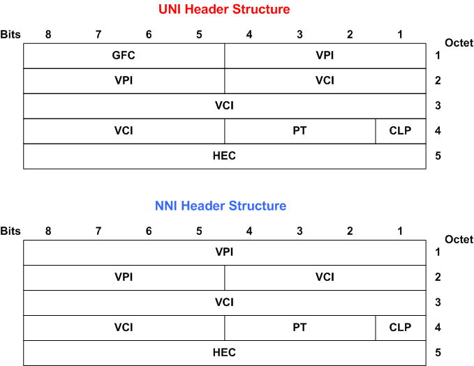
The Interface Type can be set to UNI (User-to-Network Interface) format or NNI (Network-to-Node Interface aka Network-to-Network Interface) format. The 5-byte ATM cell header is different for each of the two interfaces, as shown in Figure 2-31 on page 2-43.
Figure 2-31. ATM Cell Header for UNI and NNI
ATM OAM Cells
OAM cells are used for operation, administration, and maintenance of ATM networks. They operate on ATM's physical layer and are not recognized by higher layers. Operation, Administration, and Maintenance (OAM) performs standard loopback (end-to-end or segment) and fault detection and notification Alarm Indication Signal (AIS) and Remote Defect Identification (RDI) for each connection. It also maintains a group of timers for the OAM functions. When there is an OAM state change such as loopback failure, OAM software notifies the connection management software.
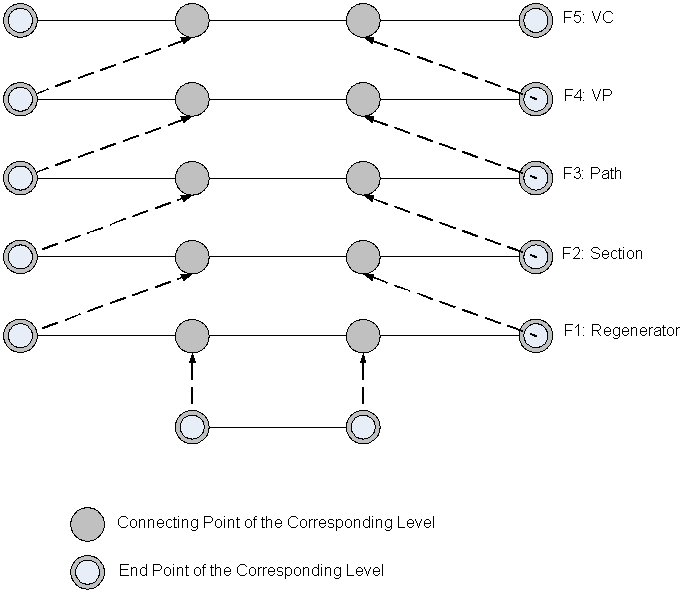
The ITU-T considers an ATM network to consist of five flow levels. These levels are illustrated in Figure 2-32 on page 2-44.
Figure 2-32. Maintenance Levels
The lower three flow levels are specific to the nature of the physical connection. The ITU-T recommendation briefly describes the relationship between the physical layer OAM capabilities and the ATM layer OAM.
From an ATM viewpoint, the most important flows are known as the F4 and F5 flows. The F4 flow is at the virtual path (VP) level. The F5 flow is at the virtual channel (VC) level. When OAM is enabled on an F4 or F5 flow, special OAM cells are inserted into the user traffic.
Four types of OAM cells are defined to support the management of VP/VC connections:
- Fault Management OAM cells. These OAM cells are used to indicate failure conditions. They can be used to indicate a discontinuity in VP/VC connection or may be used to perform checks on connections to isolate problems.
- Performance Management OAM cells. These cells are used to monitor performance (QoS) parameters such as cell block ratio, cell loss ratio and incorrectly inserted cells on VP/VC connections.
- Activation-deactivation OAM cells. These OAM cells are used to activate and deactivate the generation and processing of OAM cells, specifically continuity check (CC) and performance management (PM) cells.
- System management OAM cells. These OAM cells can be used to maintain and control various functions between end-user equipment.Their content is not specified by I.610, and they are limited to end-to-end flows.
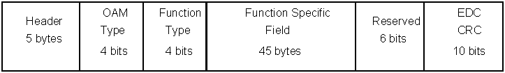
The general format of an OAM cell is shown in Figure 2-33 on page 2-45.
Figure 2-33.
OAM Cell Format
The header indicates which VCC or VPC an OAM cell belongs to. The cell payload is divided into five fields. The OAM-type and Function-type fields are used to distinguish the type of OAM cell. The Function Specific field contains information pertinent to that cell type. A 10 bit Cyclic Redundancy Check (CRC) is at the end of all OAM cells. This error detection code is used to ensure that management systems do not make erroneous decisions based on corrupted OAM cell information.
Ixia ATM modules allows to configure Fault Management and
Activation/Deactivation OAM Cells.BERT
Bit Error Rate Test (BERT) load modules are packaged as both an option to OC48, POS, and 10GE load modules and as BERT-only load modules. As opposed to all other types of testing performed by Ixia hardware and software, BERT tests operate at the physical layer, also referred to as OSI Layer 1. POS frames are constructed using specific pseudo-random patterns, with or without inserted errors. The receive circuitry locks on to the received pattern and checks for errors in those patterns.
Both unframed and framed BERT testing is available. Framed testing can be performed in both concatenated and channelized modes with some load modules.
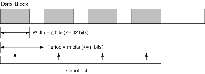
The patterns inserted within the POS frames are based on the ITU-T O.151 specification. They consist of repeatable, pseudo-random data patterns of different bit-lengths which are designed to test error and jitter conditions. Other constant and user-defined patterns may also be applied. Furthermore, you may control the addition of deliberate errors to the data pattern. The inserted errors are limited to 32-bits in length and may be interspersed with non-errored patterns and repeated for a count. This is illustrated in Figure 2-34 on page 2-46. In the figure, an error pattern of n bits occurs every m bits for a count of 4. This error is inserted at the beginning of each POS data block within a frame.
Figure 2-34. BERT Inserted Error Pattern
Errors in received BERT traffic are visible through the measured statistics, which are based on readings at one-second intervals. The statistics related to BERT are described in the Available Statistics appendix associated with the Ixia Hardware Guide and some other manuals.
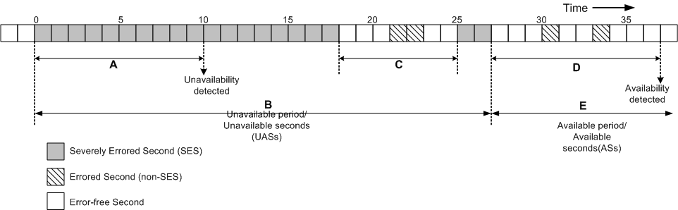
Available/Unavailable Seconds
Reception of POS signals can be divided into two types of periods, depending on the current state—`Available' or `Unavailable,'—as shown in Figure 2-35 on page 2-46. The seconds occurring during an unavailable period are termed Unavailable Seconds (UAS); those occurring during an available period are termed Available Seconds (AS).
Figure 2-35. BERT—Unavailable/Available Periods
These periods are defined by the error condition of the data stream. When 10 consecutive SESs (A in the figure) are received, the receiving interface triggers an Unavailable Period. The period remains in the Unavailable state (B in the figure), until a string of 10 consecutive non-SESs is received (D in the figure), and the beginning of the Available state is triggered. The string of consecutive non-SESs in C in the figure was less than 10 seconds, which was insufficient to trigger a change to the Available state.
Port Transmit Capabilities
The Ixia module ports format data to be transmitted in a hierarchy of structures:
- Streams and Flows—A set of related packet bursts
- Bursts and the Inter-Burst Gap (IBG)—A repetition of packets
- Packets and the Inter-Packet Gap (IPG)—Individual packets/frames
Timing of transmitted data is performed by the use of inter-stream, -burst, and -packet gaps. Ethernet modules use all three types of gaps, programmed to the resolution of their internal clocks. POS modules gaps are implemented by use of empty frames and the resolution of the gap is limited to a multiple of such frames. ATM modules do not use inter-stream or inter-packet gaps, and instead control the transmission rate through empty frames. The three types of gaps are discussed in:
The percentage of line rate usage for ports is determined using the following formula:
(packet size + 12 byte IPG + requested preamble)/
(packet size + requested IPG + requested preamble) * 100
Streams and Flows
The Ixia system uses sophisticated models for the programming of data to be transmitted. There are two general modes of scheduling data packets for transmission:
- Sequential: The first configured stream in a set of streams is transmitted completely before the next one is sent, and so on, until all of the configured streams have been transmitted. Two types are available:
- Packet Flows (available on certain modules)
- Interleaved: The individual packets in the streams are multiplexed into a single stream, such that the total packet rate is the sum of the packet rates for each of the streams. One type is available:
- Advanced Streams (Advanced Stream Scheduler feature)
ATM modules support up to 15 independent stream queues, each of which may contain multiple streams. Up to 4096 total streams may be defined. See Stream Queues on page 2-49.
Packet Streams
This sequential transmission model is supported by the Ixia load modules, where dedicated hardware can be used to generate up to 255 Packet Streams `on-the-fly,' with each stream consisting of up to 16 million bursts of up to 16 million packets each. Transmission of the entire set of packet streams may be repeated continuously for an indefinite period, or repeated only for a user-specified count. The variability of the data within the packets is necessarily generated algorithmically by the hardware transmit engine.
Packet Flows
A second sequential data transmission model is supported by software for any Ixia port which supports Packet Flows. An individual packet flow can consist of from 1 to 15,872 packets. For packet flows consisting of only one unique packet each, a maximum of 15,872 individual flows can be transmitted. Because the packets in each of the packet flows is created by the software, including User Defined Fields (UDF) and checksums, and then stored in memory in advance of data transmission, there can be more unique types of packets than is possible with streams. Continuous transmission cannot be selected for flows, but by using a return loop, the flows can be retransmitted for a user-defined count.
Packet streams, which can contain larger amounts of data, are based on only one packet configuration per stream. In contrast, many packet flows can be configured for a single data transmission, where each flow consists of packets with a configuration unique to that flow. Some load modules permit saving/loading of packet flows.
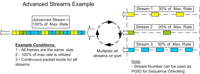
Advanced Streams
A third type of stream configuration is called Advanced Streams, which involves interleaving of all defined streams for a port into a single, multiplexed stream. Each stream is assigned a percentage of the maximum rate. The frames of the streams are multiplexed so that each stream's long-term percentage of the total transmitted data rate is as assigned. When the sum of all of the streams is less than 100% of the data rate, idle bytes are automatically inserted into the multiplexed stream, as appropriate.
Figure 2-36. Example of Advanced Stream Generation
Stream Queues
Stream queues allow standard packet streams to be grouped together. Up to 15 stream queues may be defined, each containing any number of streams so long as the total number of streams in all queues for a port does not exceed 4,096. Each queue is assigned a percentage of the total and traffic is mixed as in advanced streams. Each queue may represent any number of VPI/VCI pairs; the VPI/VCI pairs may also be generated algorithmically.
Basic Stream Operation
When multiple transmit modes are available, the transmit mode for each port must be set by you to indicate whether it uses streams, flows, or advanced stream scheduling. The programming of sequential streams or flows is according to the same programming model, with a few exceptions related to continuous bursts of packets. Since the model is identical in both cases, we refer to both streams and flows as `streams' while discussing programming.
There are three basic types of sequential streams:
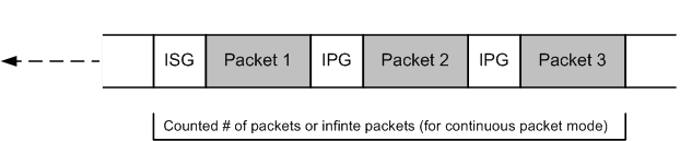
- Continuous Packet: A continuous stream of packets. The packets are not necessarily identical; their contents may vary significantly. (Not available for packet flows.)
- Continuous Burst: A set of counted packets within a burst; the burst is repeated continuously. (Not available for packet flows.)
- Counted Burst (non-continuous): A user-specified number of bursts per stream, where each burst contains a counted number of packets.
Each non-continuous stream is related to the next stream by one of four modes:
- Stop after this stream: Data transmission stops after the completion of the current stream. (For example, after transmission of a stream consisting of 10 bursts of 100 packets each.)
- Advance to Next: Data transmission continues on to the next stream after the completion of the current stream.
- Return to ID: After the completion of the current stream, a previous stream (designated by its Stream ID) is retransmitted once, and then transmission stops.
- Return to ID for Count: After the completion of the current stream, a previous stream (designated by its Stream ID) is retransmitted for the user-specified number of times (count), and then transmission stops.
If a Continuous Packet or Continuous Burst stream is used, it becomes the last stream to be applied and data transmission continues until a Stop Transmit operation is performed.
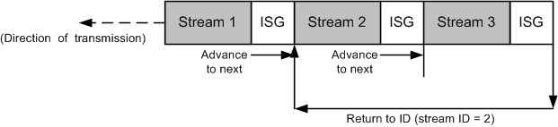
Streams and the Inter-Stream Gap (ISG)
A programmable Inter-Stream Gap (ISG) can be applied after each stream, as pictured in Figure 2-37 on page 2-50.
Figure 2-37. Inter-Stream Gap (ISG)
The size and resolution of the Inter-Stream Gaps depends on the particular Ixia module in use. For all modules except 10 Gigabit Ethernet modules, the stream uses the parameters set in the following stream. In 10 Gigabit Ethernet modules, it uses the parameters set in the preceding stream. There are no ISGs before Advanced Scheduler Streams. For non-Ethernet modules, the ISG is implemented by use of empty frames and the resolution of the ISG is limited to a multiple of such frames.
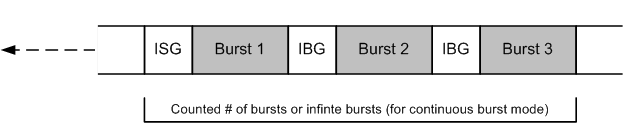
Bursts and the Inter-Burst Gap (IBG)
Bursts are sets of a specified number of packets, separated by programmed gaps between the sets. For Ethernet modules, Inter-Burst Gaps (IBG) are inserted between the sets. For POS modules, bursts of packets are separated by Burst Gaps. ATM modules do not insert IBGs. The size and resolution of these gaps depends on the type of Ixia load module in use. The placement of Inter-Burst Gaps is shown in Figure 2-38 on page 2-51.
Figure 2-38. Inter-Burst Gap (IBG)/Burst Gap
Packets and the Inter-Packet Gap (IPG)
Streams may contain a counted number of frames, or a continuous set of frames when Continuous Packet mode is used. Frames are separated by programmable Inter-Packet Gaps (IPGs), sometimes referred to as Inter-Frame Gaps (IFGs). The size and resolution of the Inter-Packet Gaps depends on the particular Ixia module in use. For non-Ethernet modules, the ISG is implemented by use of empty frames and the resolution of the IPG is limited to a multiple of such frames. ATM modules do not insert IBGs.The placement of Inter-Packet Gaps is shown in Figure 2-39 on page 2-51.
Figure 2-39. Inter-Packet Gap (IPG)
Frame Data
The contents of every frame and packet are programmable in terms of structure and data content. The programmable fields are:
- Preamble or Header contents
- Ethernet modules: Preamble Size: The size and resolution depends on the particular Ixia load module used.
- POS modules: Minimum Flag and Header contents: The minimum number of flag fields to precede the packet within the POS frame and the type of encapsulation/signalling.
- ATM modules: Header contents.
- Frame size: The size and resolution depends on the particular Ixia load module used.
- Destination and Source MAC Addresses (Ethernet only): Allows the MAC addresses to be set to constants, vary randomly, or increment/decrement using a mask.
- Data generators: Five different data generators are available. These generators are listed as follows, in order of increasing priority (from top to bottom). The values from generators located lower in this list override data from those higher in the list.
- Protocol-related data: Formatted to correspond to particular data link, transport, and protocol conventions.
- Data link layer controls for Ethernet allow for Ethernet II/SNAP, 802.3 Raw and 802.3 IPX formatting, with support for VLANs, MPLS, and Cisco-proprietary ISL. VLANs are described in Virtual LANs on page 2-52
- Protocol-specific data for formatting IPv4, IPv6, and IPX packets (such as Source and Destination IP addresses), as well as Layer 4 transport protocol headers (TCP/IP, IGMP, and so on) are also supported. IPv4/IPv6 and IPv6/IPv4 tunneling is also supported.
- IP Source and Destination addresses may be incremented or decremented using a network mask.
- Data Patterns: Can be one of three types: predefined patterns up to 8K bytes in length, randomly generated data, algorithmically generated data, industry standard (such as CJPAT and CRPAT) or user-specified.
- User Defined Fields (UDFs): A number of 32-bit counters. For some modules the counters can each be flexibly configured as multiple 8, 16, 24, and 32-bit counters. Each counter may independently increment or decrement using a mask. These are further described in User Defined Fields (UDF) on page 2-55.
- Frame Identity Record (FIR): An identity record stored at the end of the packet. The information is very useful for determining the source of transmitted data found in capture buffers.
- Frame Check Sequence (FCS): The checksum for a packet may be omitted, formatted correctly, or have deliberate errors inserted. Deliberate errors include incorrect checksum, dribble errors, and alignment errors.
Virtual LANs
Virtual LANs (VLANs) are defined in IEEE 802.1Q, and can be used to create subdomains without the use of IP subnets. The IEEE 802.1Q specification uses the explicit VLAN tagging method and port-based VLAN membership. Explicit tagging involves the insertion of a tag header in the frame by the first switch that the frame encounters. This tag header indicates which VLAN the packet belongs to. A frame can belong to only one VLAN.
VLAN tag headers are inserted into the frames, following the source MAC address. A maximum of 4094 VLANs can be supported, based on the length of the 12-bit VLAN ID. The VID value is used to map the frame into a specific VLAN. VLAN IDs 0 and FFF are reserved. VID = 0 indicates the null VLAN ID, which means that the tag header contains only user priority information.
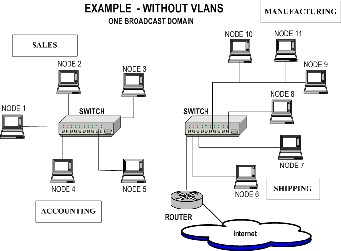
An example of Layer 2 broadcast domain without VLANs is shown in Figure 2-40 on page 2-53.
Figure 2-40. Example of Broadcast Domain Without VLANs
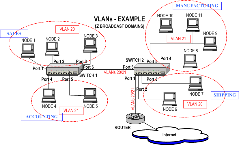
In the example above, a company has four departments (Sales, and so forth) which are in one switched broadcast domain. Broadcasts are flooded to all of the devices in the domain. A router sends/receives Internet traffic. In Figure 2-41 on page 2-54, the departments have been grouped into two separate VLANs, cutting down on the amount of broadcast traffic. For example, VLAN 20 contains Ports 1, 2, 3, and 6 on Switch 1, and Ports 1, 2, 3, and 6 on Switch 2. VLAN 21 contains Ports 4, 5, and 6 on Switch 1, and Ports 1, 4, 5, and 6 on Switch 2.
Figure 2-41. Example of VLANs
With the new network design, switch ports and attached nodes are assigned to VLANs. Frames are tagged with their VLAN ID as they leave the switch, en route to the second switch. The VLAN ID indicates to the second switch which ports to send the frame to. The VLAN tag is removed as the frame exits a port belonging to that VLAN, on its way to the attached node. With VLANs, bandwidth is conserved, and security is improved. Communication between the VLANs is handled by the existing Layer 3 router.
Stacked VLANs (Q in Q)
VLAN Stacking refers to a mechanism where one VLAN (Virtual Local Area Network) may be encapsulated within another VLAN. This allows a carrier to partition the network among several networks, while allowing each network to still utilize VLANs to their full extent. Without VLAN stacking, if one network provisioned an end user into `VLAN 1,' and another network provisioned one of their end users into `VLAN 1,' the two end users would be able to see each other on the network.
VLAN stacking solves this problem by embedding each instance of the 802.1Q VLAN protocol into a second tier of VLANs. The first network is assigned a `Backbone VLAN,' and within that Backbone VLAN a unique instance of 802.1Q VLAN tags may be used to provide that network with up to 4096 VLAN identifiers. The second network is assigned a different Backbone VLAN, within which another unique instance of 802.1Q VLAN tags is available.
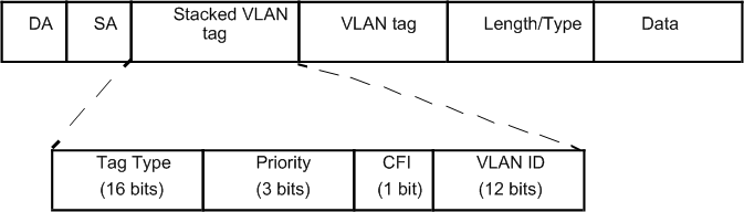
Figure 2-42 on page 2-55 demonstrates an example packet of a stacked VLAN.
Figure 2-42. Stacked VLAN Header Information
User Defined Fields (UDF)
Seven different types of UDFs are available, depending on the load module type. The types of UDFs that are supported by particular port types is detailed in Chapter 1, Platform and Reference Overview. Not all features supported by a port type are available on all UDFs; whether a particular UDF type is supported on a particular UDF can be ascertained by looking at the UDF with IxExplorer or programatically using the Tcl API. These types are:
Some features are common across all UDFs:
- Counter Type: The size of the counter is available in two modes:
- A single counter with a length of 8, 16, 24 or 32 bits, or
- A 32-bit value that may be divided into one to four 8 to 32 bit counters in any order. For example, 8x8x8x8 (four 8-bit counters), 8x16 (an 8-bit counter followed by a 16 bit counter), or 24x8 (a 24-bit counter followed by an 8-bit counter). In this case, each of the up to four counters may be independently controlled as described in Counter Mode UDF.
- Offset: The offset from the beginning of the packet to the start of the counter.
- Init val: The initial value given to the counter.
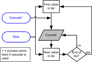
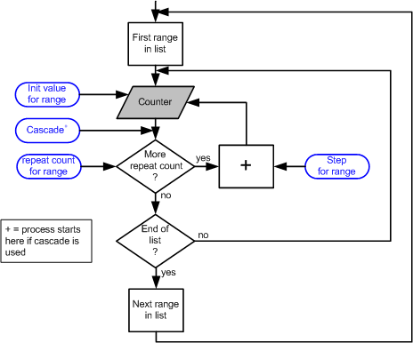
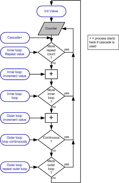
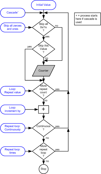
- Cascade: Sets the initial value for the counter, in one of two ways:
- From the last value for this stream: The counter continues from the last value generated by this UDF for this stream. The first value for the counter is set from the Init val setting. This type of cascade is sometimes referred to as Cascade From Self.
- From the last value on the previous cascade stream: The counter continues from the last value generated by the last executed stream using this UDF that is also in this cascade mode. The first value for the first UDF is set from the Init val setting. This type of cascade is sometimes referred to as Cascade From Previous Stream.
- Masking: The bit masking operation allows certain bits to maintain constant values, while varying other values. In the IxExplorer GUI, a bit mask is represented as a string of characters, one character per counter bit. For example, a possible Bit Mask setting for an 8-bit counter might be:
0110XXXXThe `0's and `1's represent fixed values after the mask value, while the `X's are bits which vary as a result of the increment, decrement or random value option.
In the TCL/C++ APIs, the Bit Mask value is split into two variables:
In all of the UDF figures, the generated counter value is shaded. The parameters are shown in ovals (blue in the online version).
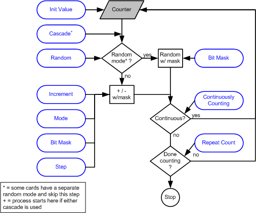
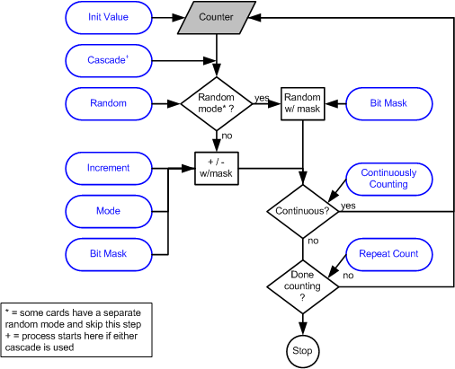
Counter Mode UDF
The counter mode UDF features the ability of a counter (up to four on some load modules) to count up or down or to use random values. Certain bits of the counter may be held at fixed values using a mask. The parameters that affect the counter's operation are shown in Table 2-12 on page 2-56.
* some card types include random mode as part of the counter mode and others use them as a separate mode.
In the TCL APIs the value of the counterMode variable in the udf command should be set to udfCounterMode (0). The operation of counter mode is described in the flowchart shown in Figure 2-43 on page 2-57.
Figure 2-43. UDF Counter Mode Operation
Random Mode UDF
The random mode UDF features a counter whose values are randomly generated, but may be masked. Cascading modes do not apply to random mode UDFs. The parameters that affect the counter's operation are shown in Table 2-13 on page 2-57.
maskselectIn the TCL APIs the value of the counterMode variable in the udf command should be set to udfRandomMode (1). The operation of random mode is described in the flowchart shown in Figure 2-44 on page 2-58.
Figure 2-44. UDF Random Mode Operation
Value List Mode UDF
The value list mode UDF features a counter whose values successively retrieved from a table of values. Cascading modes do not apply to value list mode UDFs. The parameters that affect the counter's operation are shown in Table 2-14 on page 2-58.
In the TCL APIs the value of the counterMode variable in the udf command should be set to udfValueListMode (2). The operation of value list mode is described in the flowchart shown in Figure 2-45 on page 2-59.
Figure 2-45. UDF Value List Mode Operation
Range List Mode UDF
The range list mode UDF features a counter whose values are generated from a list of value ranges. Each range has an initial value, repeat count, and step value. Cascading modes do not apply to range list mode UDFs. The parameters that affect the counter's operation are shown in Table 2-15 on page 2-59.
In the TCL APIs the value of the counterMode variable in the udf command should be set to udfRangeListMode (4). The initval, repeat, and step values are added into the udf command by the addRange sub-command. The operation of range list mode is described in the flowchart shown in Figure 2-46 on page 2-60.
Figure 2-46. UDF Range List Mode Operation
Nested Counter Mode UDF
The nested counter mode UDF features a counter whose values are generated from three nested loops:
The parameters that affect the nested counter's operation are shown in Table 2-16 on page 2-60.
In the TCL APIs the value of the counterMode variable in the udf command should be set to udfNestedCouterMode (3). The operation of range list mode is described in the flowchart shown in Figure 2-46 on page 2-60.
Figure 2-47. UDF Nested Counter Mode Operation
IPv4 Mode UDF
The IPv4 counter mode UDF features a counter designed to be used with IPv4 addresses. The process is:
- A given value may be repeated a number of times. Values with all `1's and `0's in a particular part of the value may be skipped so as to avoid broadcast addresses. The number of low order bits to check for `0's and `1's can be set.
- That value is incremented and step 1 is repeated continuously or for a count.
The parameters that affect the counter's operation are shown in Table 2-17 on page 2-62.
The operation of IPv4 mode is described in the flowchart shown in Figure 2-46 on page 2-60.
Figure 2-48. UDF IPv4 Mode Operation
Table Mode UDF
Table UDFs allows to specify a number of lists of values to be placed at designated offsets within a stream. Each list consists of an Offset, a Size, and a list of values.
Figure 2-49 on page 2-64 illustrates the basic operation of the Table UDFs using a GRE encapsulated packet as an example. Four of the fields in the packets need to be modified on a packet by packet basis—the key and sequence GRE fields and the source and destination IP addresses in the IP header. The Table UDF provides a means by which lists are developed for each of these fields and the list is associated with an offset and size within the packet. During stream generation, all lists are applied at the same time in lock step.
Figure 2-49. Table UDF Mode
A Table UDF is applied before, and can be combined with, the standard UDF fields already available on ports. By combining these two features you can model multiple flows using the powerful combination of a value list group for flow identity fields and UDFs for protocol related timestamp/sequence fields.
Table Mode UDF has a limitation compared to the other UDFs. Specifically, Table Mode behaves differently when Random Data payload is enabled for the frame.
Most UDFs are attached to the frame after the Random Data is placed in the frame; the UDFs `overlay'on top of the random data. The Table Mode UDF data, however, is put in the frame before the random data. As a result, the payload is random only after the Table UDF.
For example, if a frame has a Table UDF that is 1 byte wide starting at offset 100, random data cannot appear in the payload until byte 101. Thus, the first 100 of these frames would have the same `random' data appear within the first 99 bytes of the payload—for all 100 frames. The data would truly appear random starting at byte 101, after the Table UDF insertion.
This is the same limitation currently for random data packets that have PGID or Data Integrity enabled.
The parameters that affect the counter's operation are shown in Table 2-18 on page 2-65.
Transmit Operations
The transmit operations may be performed across any set of chassis, cards, and ports specified by you. These operations are described in Table 2-19 on page 2-65.
Repeat Last Random Pattern
The 10 GE LSM module transmit engine has the ability to provide repeatable random values in all its random number generators. This feature allows to run tests with random parameters such as frame size, frame data, and UDF values to rerun the tests with the same set of random data if a problem is found. A check box on the Port Properties transmit tab is used to enable/disable, repeating the last seed used on the port. In addition to the check box, there is a read-only window showing the last 32 bit master seed value used in generating seeds for all random number generators on the port.
Port Data Capture Capabilities
Most ports have an extensive buffer which may be used either to capture the packet data `raw' as it is received, or to categorize it into groups known as Port Groups. Each port must be designated to have a Receive mode which is either Capture or Packet Groups. Packet groups are used in measuring latency.
The start of capture buffering may be triggered by a set of matching conditions applied to the incoming data, or all data may be captured. Packets can be filtered, as well. During capture mode operation, the amount of data saved in the capture buffer can be limited to a user-defined `capture slice' portion of each incoming packet, rather than the entire packet.
Each port's Capture trigger and filter conditions are based on:
Continuous Versus Trigger Capture
For some load modules, there are more advanced options provided for setting up data capture operations on a port. These options are set in the receive mode dialog for the port. The available options are described in the following list:
- Continuous Capture. Options are as follows:
- Trigger Capture:
- Capture operation starts before a packet matching the user-defined Trigger condition is received. Options are:
- Capture operation starts after a packet matching the user-defined Trigger condition is met. Options are:
- Trigger Position: The slider bar is used to set the position (% transmitted) in the data stream where the Capture Trigger is first applied to incoming packets.
Port Capture Operations
The data capture operations may be performed across any set of chassis, cards, and ports defined by you. These operations are described in Table 2-20 on page 2-68.
Forced Collision Operation
In addition to normal capture operation, forced collisions can be generated on the receive side of some 10/100/1000 load module ports, but only when the port is in half-duplex mode.
Forced collisions operate by generating `collision' data as information is being received on the incoming port. The `collision' takes the form of a number of nibbles inserted at a user-specified offset within a packet as it is received. A period with a number of consecutive `collisions' is followed by a period with no collisions. This combination of collisions and non-colliding periods can be repeated indefinitely, or repeated for a user-specified number of times. These parameters are shown in Figure 2-50 on page 2-69.
Figure 2-50. Forced Collisions
Packet Group Operation
Packet groups are sets of packets which have matching tags, called Packet Group IDs. Real-time latency measurements within packet groups depend on coordination between port transmission and port reception. Each transmitted packet must include an inserted 4-byte packet `group signature' field, which triggers the receiving port to look for the packet group ID. This allows the received data to be recognized and categorized into packet groups for latency analysis.
Packet group IDs should be used to group similar packets. For example, packet groups can be used to tag packets connected to individual router ports. Alternatively, packet groups may be used to tag frame sizes. Such groupings allow to measure the latency with respect to different characteristics (for example, router port number or frame size as in the above scenario).
After packet group operation is triggered on the receiving port, the packet group ID—a 2-byte field which immediately follows the signature—is used as an index by the port's receive buffer to store information related to the latency of the packet. When packet group signatures and packet group IDs are included in transmitted data, an additional time stamp is automatically inserted into the packet. Figure 2-51 on page 2-69 shows the fields within packets which are important for packet grouping and latency analysis.
Figure 2-51. Packet Format for Packet Groups/Latency
A special version of packet groups, known as wide packet groups, uses a 4-byte packet group ID, of which only the low order 17 bits are active. A mask may be applied to the matching of the packet group ID. Latency, sequence checking, and first/last timestamps are supported at the same time. Latency over time and data integrity checking are not supported in this mode. Frames must be greater than or equal to 64 bytes.
Split Packet Group Operation
Split PGID allows the 32-bit PGID field used to identify and group packets to be generated from a concatenation of three separate PGID fields. Note that the method for detecting and determining if a packet has a valid signature is no different from standard PGID operation. A valid signature is still required before the concatenated PGID is considered to be valid.
Instead of having one PGID offset value with one mask, you are allowed to enter up to three separate PGID offsets and masks. The split PGID method works with both the standard instrumentation method or the floating instrumentation method, and does not interfere with other features such as time bins and bin by latency.
In addition to having three 16 bit offset values and three 32 bit mask values, the following possibilities are available for the PGID offset:
The definition of the mask is also different when in split PGID mode. In the standard PGID mode, the mask is only used to zero out PGID values and not to change the width of the final PGID. In split PGID mode, the mask is used to reduce the overall width of the PGID value for that region. A value of 1 in mask field indicates the bit is discarded (masked out).
The final 32 bit PGID value used is a concatenation of the values extracted based on the offset/mask combinations provided for the three PGID regions. The final 32 bit PGID is generated by concatenating the three regions as follows: PGID3, PGID2, and PGID1. If the concatenation of the three regions is not sufficient to fill the 32 bit value, a padding of 0 is used on the remaining leftmost bits.
Figure 2-52 on page 2-71 demonstrates the three options when employing split PGIDs.
Figure 2-52. Split PGID Scenarios
Latency/Jitter Measurements
Latency and Jitter can be measured when packet groups are enabled on a transmitting port and received on a port enabled to receive packet groups. The difference between the received time and the transmitted time held in the packet's time stamp is the measured latency or jitter. The latency is included in a memory cell indexed by the packet group ID. The count of packets received, minimum, maximum, average, and mean latencies are maintained. There are two modes for latency measurement:
- Instantaneous: Latency measured for all received data (continuous). The number of PGID groups available depends on the features being employed on the receive side. The PGID is used as an index into an area of cells and the count/min/max/avg/mean is maintained for each PGID.
- Latency over time: Latency measured for a number of time intervals of equal length, called `time buckets.' The range of cells is divided up over a period of time—for example, for one second intervals over a 30 second period. Each time period (one second in this example) is called a time bucket. Within each time bucket, the data for all PGIDs must be stored into a limited number of cells. This is accomplished by grouping a number of PGIDs together. The grouping is called the `# of PGIDs/Time Bucket'. Figure 2-53 on page 2-72 demonstrates the relationship between the time buckets and PGIDs in an example. The minimum size time bucket varies by port type, but the size set should be reasonable for the transmission speed of the port—certainly no shorter than 1 microsecond.
Figure 2-53. Multiple Latency Time Measurements—Example
The timeline is equally divided into a # of Time Buckets, each of which is one Time Bucket Duration in length. A time bucket duration can range anywhere from nanoseconds to hours, depending on the user configuration.
The maximum number of time buckets that can be handled is determined by the number of PGIDs in each bucket.
Four types of timing measurements are available, corresponding to the type of device under test:
- Cut-Through: For use with switches and other devices that operate using packet header information. The time interval between the first data bit out of the Ixia transmit port and the first data bit received by the Ixia receive port is measured. The first data bit received on Ethernet links (10/100 and Gigabit modules) is the start of the MAC DA field. For Packet over SONET links, the first bit received is the start of the IP header.
- Store and Forward: For use with routers and other devices that operate on the contents of the entire packet. The time interval between the last data bit out of the Ixia transmit port and the first data bit received by the Ixia receive port is measured. The last data bit out is usually the end of the FCS or CRC, and the first data bit received is as described above for Cut Through.
NOTE: Store and Forward latency mode is intended to test Store and Forward switching devices, which receive the entire packet before transmitting it to its destination. If Store and Forward latency is used in loopback, back-to-back or without a Store and Forward switch, then either a zero latency or very high latency is reported.- Store and Forward Preamble (only available on some load modules): As with store and forward, but measured with respect to the preamble to the Ethernet frame. In this case, the time interval between the last data bit out of the Ixia transmit port and the first preamble data bit received by the Ixia receive port is measured. For this measurement, the size of the preamble (in bytes) is considered.
- Inter-Arrival Time (IAT): Compares the time between PGID packet arrivals. In this case, when a packet with a PGID is received, the PGID is examined. If a packet has already been received with the same PGID, then the timestamp of the previous packet is subtracted from the current timestamp. The interval between the timestamps is the jitter, and it is recorded for statistical purposes.
Sequence Checking Operation
A number of ports have the additional ability to insert a sequence number at a user-specified position in each transmitted packet. This sequence number is different and distinct from any IP sequence number within an IP header. On the receiving port, this special sequence number is retrieved and checked, and any out-of-sequence ordering is counted as a sequence error.
As in packet groups (see Packet Group Operation on page 2-69), for sequence checking a signature value is inserted into the packet on the transmit side to signal the receive side to check the packet. In fact, this particular signature value is shared by both the packet group and the sequence checking operations. Both the signature value and sequence number are 4-byte quantities and must start on 4-byte boundaries. These fields are shown in Figure 2-54 on page 2-73.
Figure 2-54. Packet Format for Sequence Checking
Sequence numbers are integers which start at `0' for each port when transmission is started, and increment by `1' continuously until a Reset Sequence Index operation is performed. Note that multiple sequence errors results when a packet is received out of sequence. For example, if five packets are transmitted in the order 1-2-3-4-5 and received in the order 1-3-2-4-5, three sequence errors are counted:
Switched-Path Duplicate/Gap Checking Mode
This is a mode in sequence checking that allows for detecting duplicate packets, or sequence gaps. IxExplorer stores the largest sequence number received. Any packet that arrives with a lower or equal sequence number is regarded as a duplicated packet. For a flow with no packet reordering, the `reversal errors' matches the number of duplicates received. For a flow with packet reordering, the `reversal errors' gives a count that may be higher than the number of duplicates received.
Data Integrity Checking Operation
A number of ports also possess the ability to check the integrity of data contained in a received packet, by computing an additional 16-bit CRC checksum.
As with packet groups (see Packet Group Operation on page 2-69) and sequence checking (see Sequence Checking Operation on page 2-73), a signature value is inserted into the packet on the transmitting interface, to serve as a trigger for the receiving port to notice and process the additional checksum. The data integrity operation uses a different signature value from the one shared by packet groups and sequence checking.
The data integrity signature value marks the beginning of the range of packet data over which the 16-bit data integrity checksum is calculated, as shown in Figure 2-55 on page 2-74. This packet data ends just before the timestamp and normal CRC/FCS. The CRC-16 checksum value must end on a 4-byte boundary. There may be 1, 2, or 3 bytes of zeroes (padding) inserted after the CRC-16, but before the Time Stamp, to enforce all boundary conditions.
Figure 2-55. Packet Format for Data Integrity Checking
When the Receive Mode for a port is configured to check for data integrity, received packets are matched for the data integrity signature value, and the additional CRC-16 is checked for accuracy. Any mismatches are recorded as data integrity errors.
Automatic Instrumentation Signature
The Automatic Instrumentation Signature feature allows the receive port to look for a signature at a variable offset from the start of frames. The feature supports Sequence Checking, Latency, Data Integrity functionality, with signature and Packet Group ID (when Automatic Instrumentation is enabled, these receive port options are enabled as well).
In normal stream operation, signatures for Data Integrity, Latency, and Sequence Checking are forced to a single, uniform offset location in each frame of the stream. Many of the Ixia software application (that is, IxVPN, IxChariot, and so forth) can generate streams that place a signature at random places within the frames of a single stream. To accurately detect these signatures on the receive side of the chassis, Automatic Instrumentation Signature is used.
Automatic Instrumentation Signature allows the chassis to look for a floating pattern in the frame. Two data blocks are placed in the frame (by some stream generating application). The first is positioned at a variable offset from the start of the frame. The second is positioned at a fixed 12 byte offset from the end of the frame.
Figure 2-56 shows the composition of the blocks.
Figure 2-56. Automatic Instrumentation Signature Block
The receive port recognizes an instrumented frame by detecting the Signature in the first block. Once a signature match has occurred, the Packet Group ID (PGID) and Sequence Number are extracted from the frame. Data Integrity also starts immediately following the signature.
The Checksum Adjust field is reserved for load modules that cannot correctly do checksums on large frames.
Port Transmit/Receive Capabilities
Round Trip TCP Flows
For most 10/100 load modules, a special capability exists in the Ixia hardware to enable the measurement of round trip times for IP packets sent through a switch or other network device. The normal setup for this measurement is shown in Figure 2-57 on page 2-75.
Figure 2-57. RoundTrip TCP Flows Setup
In this scenario, Ports A and X are configured on one IP subnet, and Ports B and Y are configured on a different IP subnet. IP packets sent from A have a source address of A and destination address of B. The DUT is configured to route or forward to Y any packets that it receives on X for an address on B-Y's subnet. After being received on Port B, the packet is reconstructed in a modified form as described in the following list, and sent back in the opposite direction along the path to Port A.
When enabled on the Ixia receiving port (in this case, Port B), the Round Trip TCP Flows feature performs several operations on the received IP packet:
- The Source and Destination IP addresses are reversed, and a packet destined for Port A is created using the reversed addresses.
- The frame size, source and destination MAC addresses, and background data pattern are set as specified by you.
- The timestamp is copied to the new packet unmodified.
- The new packet is transmitted to Port Y on the DUT, and should be routed back to Port A by the DUT.
This re-assembly/retransmit process makes it possible to measure the round-trip time for the packet's trip from Port A through the DUT to Port B, and back through the DUT to Port A again. Note that the Packet Groups feature may be used, in addition, for latency measurements on this round trip. For latency testing, the background data set by the Round Trip TCP Flows feature overwrites the Packet Group Signature Value contained in the packet. It is important that proper programming of the background data pattern be used to insert the appropriate signature value back into the packet.
Port Statistics Capabilities
Each port automatically collects statistics. A wide range of statistics are preprogrammed and available for many types of load modules. Other statistics may be selected or programmed and include:
- User-Defined Statistics: Four counters which can be programmed to increment based on the same conditions as those involved in defining capture triggers and capture filters.
- Quality of Service Types: Separate counts for each of eight Quality of Service values used in IP headers.
- IP/UDP/TCP Checksum Verification Statistics: For hardware checksum verification.
- Data Integrity Statistics: For errors relating to Data Integrity Operation. Refer to Data Integrity Checking Operation on page 2-74.
- Packet Group Statistics: For statistics relating to Latency operations. Refer to Latency/Jitter Measurements on page 2-71.
- Protocol Server Statistics: Protocol-based statistics for a wide range of routing protocols.
- SONET Extended Statistics: Statistics associated with SONET Line, Section and Path characteristics.
- VSR Statistics: Statistics associated with OC192 VSR modules.
- ATM Statistics: Statistics associated with ATM modules.
- BERT Statistics: Statistics associated with BERT error generation and detection.
- Temperature Sensors Statistics: For verifying that temperatures on high-performance 10 Gigabit and OC-192c POS cards are within operational limits.
IxExplorer Software
The IxExplorer software utilizes concepts that match the Ixia hardware hierarchy. The software hierarchy is:
- Chassis Chain (Software): A set of Ixia chassis joined through sync-in/sync-out cables.
- Chassis: A single Ixia chassis capable of holding different Ixia module cards.
- Card: An Ixia module card, all of whose ports have the same features.
- Port: An individual transmit/capture port on a card.
- Capture View: A view of the capture buffer for the port.
- Filters, Statistics and Receive Mode: A means of programming capture triggers, filters, and statistics.
- Packet Streams: A means of programming sets of streams and flows.
- Statistics: A view of the statistics gathered by the port.
- Global Views:
- Port Groups: Hold groups of related ports that may be operated on at the same time.
- Stream Groups: Hold groups of related ports that may be operated on at the same time.
- Packet Group Statistic Views: Allows the latency data (including Inter-Arrival Time) to be collected from one or more ports that are configured to receive packet groups.
- Statistic Views: Holds groups of related ports, all of whose statistics can be viewed at one time.
- Stream Statistic Views: Holds groups of related streams, all of whose statistics can be viewed at one time.
- MII Templates: A means of creating and editing MII templates.
- Layouts: A means of saving open GUI features.
- IxRouter Window: A means of designating interface addresses associated with ports and programming routing protocol simulations on each port. Note that IxRouter must be installed for full use of this window. Without IxRouter, only limited use of ARP and PING are allowed. See IxRouter User Guide for more information.
Chassis Chain (Software)
The IxExplorer chassis chain corresponds to the hardware chain. The chain starts with a master, whose sync-out line is connected to the sync-in line of the next chassis, and so on. Multiple chassis chains may be defined in the IxExplorer and operated independently or at the same time. Various forms of time synchronization may be used to coordinate multiple chassis chains dispersed world-wide into a single `virtual chassis chain'; see Chassis Synchronization on page 2-5. The Ixia 100 chassis includes a built-in GPS receiver to provide very accurate timing.
Chassis
The IxExplorer chassis corresponds to an Ixia 1600T, 400T, 250, 100, Optixia XL10, Optixia XM12, Optixia XM2, Optixia X16 or other chassis capable of holding Ixia module cards. The name or IP address of each chassis must be input; the type of the chassis is automatically discovered by the software. A chassis may hold any mix of module cards.
Card
The IxExplorer card corresponds to an Ixia load module card. The types of cards loaded in a chassis are automatically discovered and the appropriate number of ports are inserted into the hierarchy. Each port on a card has the same capabilities.
Port
The IxExplorer port corresponds to an individual port on an Ixia module card. Each port is independently programmed in terms of its transmit, capture and statistics capabilities. The IxExplorer software shows four separate views for programming and viewing operations:
- Filters, Statistics and Receive Mode: Sets the trigger and capture conditions for the capture buffer, conditions for the four user-defined statistics, and the receive mode for the port.
- Packet Streams/Flows: Defines the streams within stream regions and the contents of packets.
- Capture View: Shows the data gathered during capture operations. Data is displayed in raw form and interpreted for some protocols.
- Statistics : Shows the live statistics gathered during transmit and capture operation.
Port Properties
A Port Properties dialog allows other port related properties to be programmed:
- Auto-Negotiation: Low level physical controls, such as 10 versus 100 Mbps operation and full duplex versus half duplex.
- Advanced MII controls: Additional low level MII register controls.
- Flow control: Related to pause control operation.
- Collision Backoff Algorithm: Handling of collision situations.
- Forced Collisions: The generation of collision packets on receive ports.
- Transmit mode: The choice of streams or flows for the port.
- SONET Header: For use with Packet Over SONET frames.
- SONET Overhead: For generation of APS (K1/K2), J0/J1 bytes, and Error Insertion.
- PPP: For use with SONET. Includes dialogs for Negotiation, Link Control Protocols, and Network Control Protocols.
Port Groups
Port groups are an IxExplorer convenience. They allow to perform operations, such as start/stop transmit, start/stop capture and clear timestamps, for a wide range of ports all at the same time.
Stream Groups
Stream groups are an IxExplorer convenience. They allow to perform operations, such as start/stop transmit, start/stop capture and clear timestamps, for a group of streams all at the same time.
Packet Group Statistic Views
The Packet Group Statistics View allows the latency data (including Inter-Arrival Time) to be collected from one or more ports that are configured to receive packet groups. Packets representing different types of traffic profiles can be associated with packet group identifiers (PGIDs). The receiving port measures the minimum, maximum, and average latency in real time for each packet belonging to different groups. Measurable latencies include Instantaneous Latency, where each packet is associated with one group ID only, and Latency Over Time, where multiple PGIDs can be placed in `time buckets' with fixed durations.
Statistic Views
Statistic Views are similar to port groups, in that they let you consider a set of ports all at once. When a Statistic View group is selected, all of the statistics for all of the ports are simultaneously viewed. The particular statistics viewed may be independently selected for each Statistic View. Statistic logging and alerts are also provided; see Statistics Logging and Alerts on page 2-82
Stream Statistic Views
Stream Statistic Views are like Statistic Views, but on a per stream basis rather than per port basis.
MII Templates
Allows for the creation and/or editing of MII template files. Register templates are applied to physical ports through Port Properties dialogs.
Layouts
Allows for the creation of templates for the layout of the IxExplorer GUI. A layout consists of the combined open features in the GUI.
IxRouter Window
The IxRouter window provides the means by which routing protocols are emulated by the Ixia hardware and software. This window includes the interface by which multiple IPv4 and IPv6 interfaces are associated with each port. A growing number of protocols are supported in this window, including ARP, BGP, OSPF, ISIS, RSVP-TE, LDP, RIP, RIPng, and IGMP.
Note that full use of this window requires that IxRouter be installed. For more information on protocols and protocol testing, see IxRouter User Guide.
IxExplorer Operation
IxExplorer saves all settings and programming in `saved' named files, which may be retrieved on each invocation. Captured data is lost when the IxExplorer is exited.
All IxExplorer test operations perform on an arbitrary set of ports, as single port or multiple ports may be selected. Any level of the hierarchy may be selected to include all ports below that level. For example, selecting a card includes all ports on that card, or selecting a chassis chain includes all ports on all cards in all chassis in the chassis chain. In addition, port groups may contain ports from any card; the port group may then be used in any testing operations.
The operations that can be performed on any group of ports:
- Start/Stop Capture: When capture is enabled, data for each port that is configured for capture (versus latency) is collected when the trigger is satisfied and to the extent that the filter is satisfied as well.
- Start/Stop Transmit: When transmit is enabled, data is transmitted as programmed to the extent designated by the synchronous stream region.
- Start/Stop Collision: Forced collisions are enabled/disabled for receive ports.
- Start/stop Latency: When latency measurement is enabled, data for each port configured for latency (versus capture) is collected when the trigger is satisfied and to the extent that the filter is satisfied as well.
- Pause/Single-Step Transmit: Transmittal of information may be paused and then single-stepped on a stream-by-stream basis or continued through a start transmit command.
- Interactive streams: This is a special function that allows for interactive variation of frame size and inter-packet gaps. Interactive streams may not be operated across ports that are configured for flows.
Multi-User Operation
IxExplorer provides an optional means of coordinating the sharing of chassis ports among multiple users. If a single user is operating a chassis, multi-user commands are not required at all. As an user, you may perform any operation on any port. Two or more people may also share ports on a chassis without use of IxExplorer multi-user facilities, through some verbal agreement (for example, `You take cards 1-8 and I'll take cards 9-16'). IxExplorer provides no assistance in this instance.
Where more accurate control over port sharing is required, multi-user facilities should be used. IxExplorer's multi-user model is a very simple, advisory model. Each user logs in with an arbitrary name. Each and every user may take ownership of any and all ports. A port owner has the ability to read data and program the port; all other users have read-only access to the port. A port owner may clear ownership of ports, making them available for other users. You may take ownership of a port owned by someone else, with an optional warning message. Any user may clear all ownerships.
IxExplorer provides a further distinction of roles between users. Administrators are privileged users who may take ownership of ports, configure their characteristics, and initiate tests using those ports. Operators are unprivileged users who may only look at chassis, card, and port characteristics and measured data.
The two basic modes of multi-user operation are referred to as:
- Voluntary: All users are considered administrators and voluntarily login and take or clear ownership of ports. All chassis are initially configured in this mode.
- Secure: Users are characterized as Administrators or Operators. All users must login. Administrators operate in the same manner as all Voluntary mode users. Operators are restricted to viewing data.
Statistics Logging and Alerts
IxExplorer has the ability to centrally log statistics from any port and to signal alert conditions when a particular statistic goes out of a specified, valid range. Figure 2-58 on page 2-82 shows the basic operation of logging and alerts.
Figure 2-58. Statistics Logging and Alerts
The clients (Client 1 and Client 2) run IxExplorer and are connected to all of the chassis (Chassis 1, Chassis 2 and Chassis 3) in the chassis chain. The clients set up conditions under which statistics data is logged and alerts generated. These conditions are transmitted to all of the chassis. Each chassis interprets these conditions and logs statistics data and alert conditions to their local disks.
When a chassis detects an alert condition, it sends signals to all of the clients connected to the chassis at the moment. Each client receives alerts from all of the chassis, regardless of whether they set up the particular alert condition themselves.
It can take considerable effort to set up one port's statistics logging and alert conditions. It is not necessary to repeat this process for multiple ports that have identical logging and alert behavior. IxExplorer's Port Copy feature may be used to copy these specifications.
It should be noted that logging and alerts continue even after a client has exited IxExplorer.
Statistics Logging
Each client selects particular statistics on particular ports to be logged. The data is logged at the chassis hosting the port. All clients connected to a chassis contribute their desired port-statistics to be logged. All statistics from all clients are logged to the same single file on a chassis.
The log file is ASCII in format and contains a line of text for each port on which statistics have been gathered. Each line contains all of the selected statistics for the port, separated by commas. The contents of the file are easiest to understand and interpret if the same statistics are gathered for all ports.
The statistic values that are logged are the `rolling average' for the value logged. That is, a value at time slot n depends on the previous average and the current measured value, as per the following equation:
Averagen = (Averagen-1 * (n-1)/n) + (Measurementn * 1/n)
The client specifies several parameters that affect the logging of statistics:
Multiple clients should agree on the log interval and file naming conventions; the chassis uses the settings received from any client that applies changes.
Alerts
Each client sets up anticipated valid ranges for particular statistics on specific ports. All clients connected to a chassis distribute their specific valid ranges to all chassis. Each chassis watches for out of range values on the specified port-statistics and generates alerts for the conditions. All alert conditions are sent to all connected clients. Alert condition changes may be optionally logged on files at the chassis.
The client indicates how it wants to receive alerts for a particular statistic and port. There are three options:
- Visual: each statistic subject to alerting is displayed as green (in range), red (out of range) or yellow (was previously out of range) in any Statistic View containing the port-statistic.
- Audible: while any out of range condition exists, the client's computer issues a repeating beep-beep. A client may mute all audible alarms at once.
- Both visual and audible.
In addition, the existence of an alert condition for a particular port-statistic may be used to initiate statistics logging for that port, as described in Statistics Logging on page 2-83.
The client specifies several parameters that affect the setup of alert conditions:
Multiple clients should agree on the valid range of port-statistics values and file naming conventions; the chassis uses the settings received from any client that applies changes.
Tcl Software Structure
The Tcl software is structured as a number of client-server pieces so that it may operate simultaneously in three different environments:
The following sections describe the components used in each of these scenarios.
Operation on the Ixia Chassis
When the Tcl client software is installed on the Ixia chassis itself three distinct software components are used, as shown in Figure 2-59 on page 2-85.
Figure 2-59. Software Modules Used on an Ixia Chassis
In this scenario, three components are used as described in Table 2-21.
Operation on a Windows Client
When the Tcl client software runs on a Windows client, the same three components are used but in a different configuration, as shown in Figure 2-60 on page 2-86.
Figure 2-60. Software Modules Used on a Windows Client
In this scenario, three components are used as described in Table 2-22.
Operation on a Unix Client
When the Tcl client software runs on a Unix client, five components are used as shown in Figure 2-61 on page 2-87.
Figure 2-61. Software Modules Used on a Unix Client
In this scenario, five components are used as described in Figure 2-23 on page 2-87.
Multiple Client Environment
A single Ixia chassis may be used by multiple clients simultaneously. Clients may run from the Ixia chassis, Windows clients, and Unix clients simultaneously, as shown in Figure 2-62 on page 2-88.
Figure 2-62. Multi-Client Environment
TCL Version Limitations
Note the following limitation with respect to Tcl versions and the use of Wish and Tclsh shells:
The use of the Wish shell with Ixia software has been tested for Tcl 8.3 under Windows, Linux, and Solaris. It has not been tested, but should run with any Tcl version greater than or equal to 8.2.
Beginning with the Ixia TCL libraries supplied with IxOS version 3.80, these libraries are compatible with TCL version 8.3 and above. That is, it is not necessary to obtain a new version of the Ixia libraries when TCL 8.4 (or above) is installed on a computer.
|
|
Did this document answer your question?
If not, let us know! |
|